In a previous post, I outlined my workflow for preparing maps in R. Today I had to add a graticule, a grid of latitude and longitude lines, to my maps. That’s easy enough to do with unprojected maps, as the plot coordinates are latitude and longitude, so your X and Y axes are already graticules. But if you’ve projected your data, the plot coordinates are on a different scale, so you need to do a bit of tuning.

I couldn’t find a direct way to do this in the R sp package. However, sp (sp for ‘spatial’) is slowly being replaced by sf (sf for simple feature), and sf does support graticules. Here are the steps required to add them to your plots:

Importing Data

We can use raster::getData to get our map data again. It’s straightforward to convert objects from sp (Spatial*) and sf (sf*) format and back, with the functions st_as_sf (to convert from a Spatial* to sf*), and as (to convert from sf* to a Spatial* object). As it turns out, getData also supports downloading data directly into sf format:

library(sf)
library(raster)
us <- getData("GADM", country = "USA", level = 1,
             path = "./data/maps/", type = "sf")
canada <- getData("GADM", country = "CAN", level = 1,
                 path = "./data/maps", type = "sf")
mexico <- getData("GADM", country = "MEX", level = 1,
                 path = "./data/maps", type = "sf")

This uses the undocumented type argument, set to sf. Given that it’s not documented, it may change in future, be warned!

You can also use the function st_read to read shapefiles directly:

greatlakes <- st_read("data/maps/greatlakes.shp")

## Reading layer `greatlakes' from data source 
##   `/home/smithty/blogdown/content/tutorials/data/maps/greatlakes.shp' 
##   using driver `ESRI Shapefile'
## Simple feature collection with 2 features and 5 fields
## Geometry type: POLYGON
## Dimension:     XY
## Bounding box:  xmin: -365240.6 ymin: -2741892 xmax: 1888977 ymax: 509590.2
## proj4string:   +proj=laea +lat_0=45 +lon_0=-100 +x_0=0 +y_0=0 +a=6370997 +b=6370997 +units=m +no_defs

In the previous tutorial, I used bind to combine two Spatial* objects. With sf we need rbind instead:

na <- rbind(us, canada, mexico)

## old-style crs object detected; please recreate object with a recent sf::st_crs()
## old-style crs object detected; please recreate object with a recent sf::st_crs()
## old-style crs object detected; please recreate object with a recent sf::st_crs()
## old-style crs object detected; please recreate object with a recent sf::st_crs()
## old-style crs object detected; please recreate object with a recent sf::st_crs()
## old-style crs object detected; please recreate object with a recent sf::st_crs()
## old-style crs object detected; please recreate object with a recent sf::st_crs()
## old-style crs object detected; please recreate object with a recent sf::st_crs()
## old-style crs object detected; please recreate object with a recent sf::st_crs()
## old-style crs object detected; please recreate object with a recent sf::st_crs()

Plotting complex vector maps like this can be a slow process, especially when you’re constantly tweaking and adjusting them. You can speed this up by simplifying the layers:

na.simp <- st_simplify(na, dTolerance = 0.01)

On my laptop, plotting the original map takes a minute or more, compared to 2 seconds for the simplified vector. I set the tolerance by trial and error. The higher the tolerance, the smoother the map will be. At 0.01, it still looks nearly identical at the scale I’m plotting it, but is much smaller and faster to plot. sf does warn me about not correctly simplifying the data, but since I’m only using this for display that’s not a concern. I wouldn’t simplify a vector if I was going to use it in an analysis.

Plotting Maps

When it comes to plotting, we need to tell R to plot only the geometry. By default it will plot multiple maps, one for each attribute. That’s not what we want here.

plot(st_geometry(na.simp), xlim = c(-130, -70),
     ylim = c(35, 45))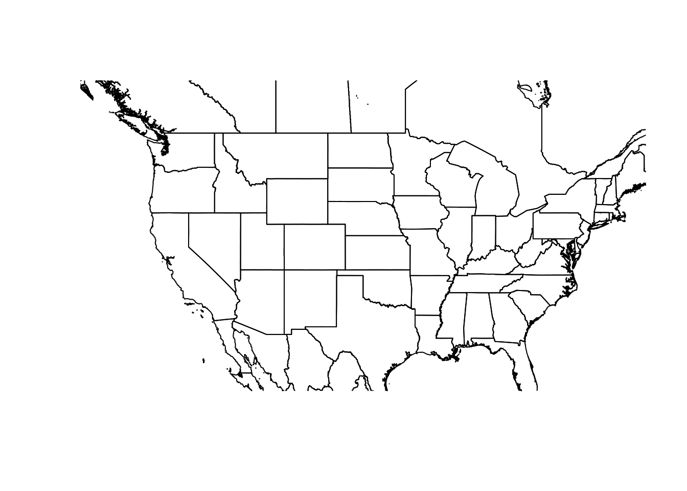

Projections

To project our unprojected data, we need to define a projection, and transform the object.

laea = CRS("+proj=laea +lat_0=30 +lon_0=-95")

## NOTE: rgdal::checkCRSArgs: no proj_defs.dat in PROJ.4 shared files

na.la <- st_transform(na.simp, laea)
plot(st_geometry(na.la), xlim = c(-500000, 2000000),
     ylim = c(-400000, 2100000))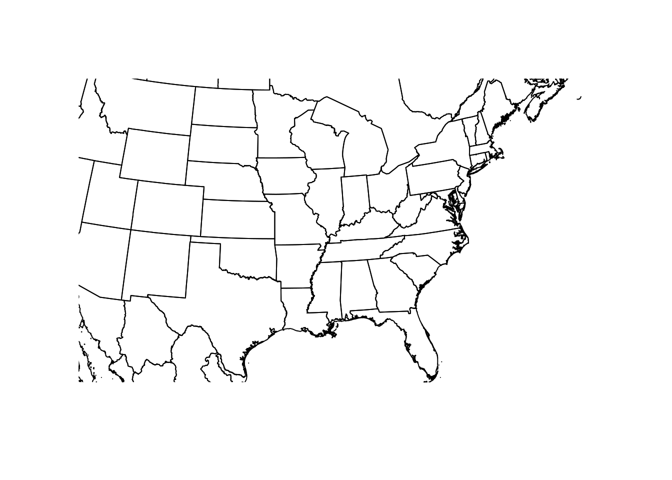

We can add layers just as we did in the previous post:

gl.la <- st_transform(greatlakes, laea)
plot(st_geometry(gl.la), col = 'lightblue', add = TRUE)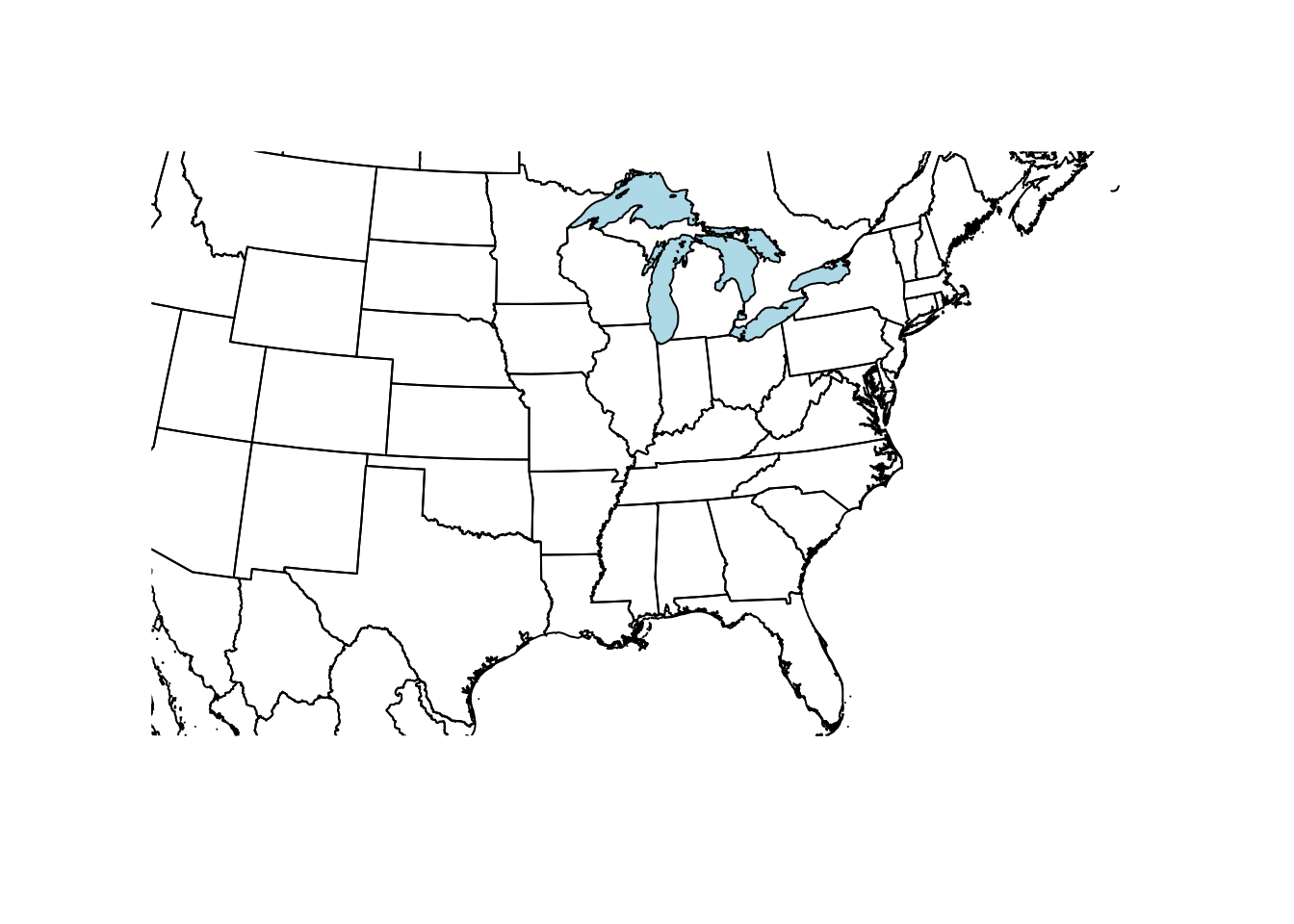

You can also mix sf and Spatial* objects on the same plot, as long as they’re in the same projection.

Graticules

Now we have everything we need to add graticules to our map. This includes the map we want to plot, and the CRS data for the graticules we want to overlay. In our case, we’ll use the original, unprojected layer as the source our CRS:

plot(st_geometry(na.la),
     xlim = c(-500000, 2000000), ylim = c(-400000, 2100000),
     graticule = st_crs(na.simp),
     bgc = 'lightblue', ## Background color for the ocean
     col = 'white',
     axes = TRUE)
plot(st_geometry(gl.la), col = 'lightblue', add = TRUE)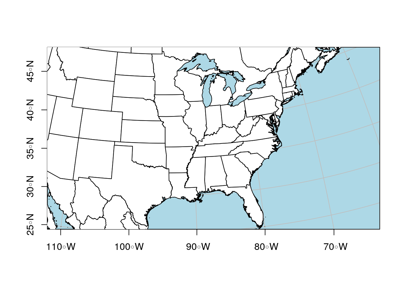

If you want to specify the location of the graticules, you can use the arguments lat and lon to specify where you want them.

Adding Lat/Lon Grids to Maps in R

Importing Data

Plotting Maps

Projections

Graticules