Background

Schoener’s D was created by Schoener (1968) He was studying the feeding niche of anoles, and needed a way to quantify the overlap in prey items for different species. This is what he came up with:

\[D(p_X, p_X) = 1 - \frac{1}{2} \sum_i \vert p_{X,i} - p_{Y, i} \vert\]

Here, \(p_{X,i}\) and \(p_{Y,i}\) are the frequencies for species \(X\) and \(Y\), respectively, for the \(i^{th}\) category. For Schoener, the categories were prey sizes. In the context of distribution modeling, they would be regions along an environmental gradient, and the ‘frequencies’ are the fitted values from an SDM, or the density values from an Ecospat dynamic niche grid.

Warren et al. (2008) pointed out some subtle theoretical issues with Schoener’s D in this context, and proposed his own index I, based on the Hellinger distance, to better account for them.

Hellinger’s distance:

\[H(p_X, p_Y = \sqrt{\sum_i(\sqrt{p_{X,i}} - \sqrt{p_{Y,i}})^2}\]

Warren’s I:

\[I(p_X, p_Y) = 1 - \frac{1}{2} H(p_X, p_Y)\]

In application, Schoener’s D suggests that the \(p_{X, i}\) values reflect relative use of a particular habitat. However, ENM predictions indicate the relative ‘suitability’ of a cell for occupancy (i.e., presence or absence) by the study species, but do not necessarily reflect density.

However, Warren also noted that despite the potential issues, in practice there is little difference in the qualitative results following from D and I. I think Schoener’s D is more commonly used now, but either or both may show up in distribution modeling studies.

Overlap vs Correlation

Warren (2018) made an interesting contrast between two species’ niche overlap (D), and the correlation between their suitability scores. Schoener’s D quantifies the extent to which a pair of species may interact in the same space (i.e., they’re both likely to be present together in a location). This is important to know, especially in the context of niche-shift studies (e.g. Atwater and Barney, 2021). But while they tell us about where species are found along an environmental gradient, they don’t tell us anything about how they respond to that gradient. In fact, species with perfectly opposite responses to the environment may still have relatively high niche overlap, D.

Let’s revisit the example from Warren (2018). We start with the olaps helper function, which calculates the statistics of interest:

library(ggplot2)
library(grid)

olaps <- function(sp1, sp2){
  ## Calculate Schoener's D, Warren's I, and Spearman
  ## Correlation for sp1 and sp2

  ## sp1 and sp2 are the relative occupancy values for each
  ## species along the same environmental gradient

  ## scale the values for each species 0:1
  sp1 <- sp1/sum(sp1)
  sp2 <- sp2/sum(sp2)
  
  plot.table <- data.frame(
    species = c(rep("sp1", length(sp1)),
                rep("sp2", length(sp2))),
    env = c(seq(1:length(sp1)), seq(1:length(sp2))),
    suitability = c(sp1, sp2))

  D = 1 - sum(abs(sp1 - sp2))/2
  I = 1 - sum((sqrt(sp1) - sqrt(sp2))^2)/2
  cor = cor(sp1, sp2, method = "spearman")

  grob <- grobTree(textGrob(paste("D =", round(D, 2),
                                 "  I =", round(I, 2),
                                 "  Cor =", round(cor, 2)),
                           x = 0.1,  y = 0.95, hjust = 0,
                           gp = gpar(fontsize = 15)))
  

  suitplot = qplot(env, suitability, data = plot.table,
                   col = species, geom = "line") +
    annotation_custom(grob)

  return(list(
    D = D, I = I, cor = cor, suitplot = suitplot
  ))
  
}

Now we can recreate the examples from Warren (2018).

sp1 <- seq(0.1, 1.0, 0.001)
sp2 <- seq(0.1, 1.0, 0.001)

olaps(sp1, sp2)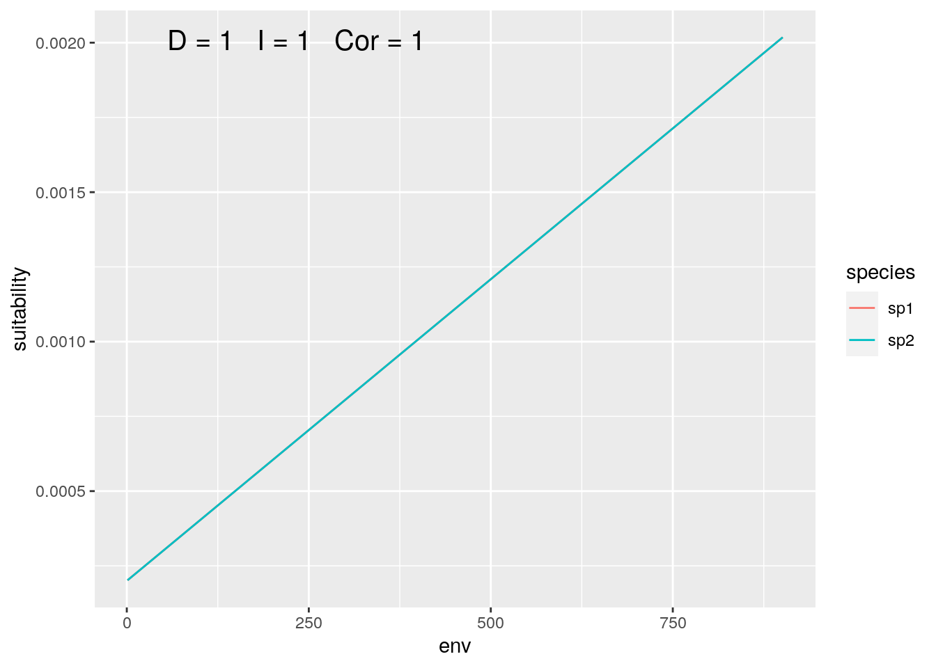

Figure 1: Identical Species

sp1 <- seq(0.1, 1.0, 0.001)
sp2 <- seq(1.0, 0.1, -0.001)

olaps(sp1, sp2)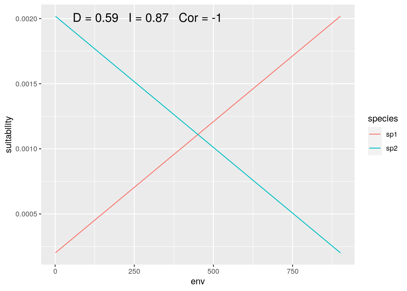

Figure 2: Species with Inverse Environmental Response

The point that Warren (2018) was making is that two species may occupy more or less similar locations along an environmental gradient, while having very different responses to that gradient. This isn’t a problem. But it does highlight the importance of clearly articulating the question you are asking in your research, and making sure that the analyses you choose are actually answering that question.

Niche Overlap vs Study Extent

Something else struck me reading Warren’s post. The toy examples he used represent a very narrow slice of an environmental gradient; that is, the portion where both species are present. Applying these analyses to global patterns, as we do when comparing the distribution of invasive species in their native and introduced range, and especially when we apply these analyses to large numbers of species, we can (potentially) include much broader gradients. And this can have significant impact on theses statistics.

Here’s a (ever so slightly) more realistic example to illustrate. We’ll define our gradient over the range 0 to 50

env <- seq(0, 50, by = 0.01)

Then we’ll define two species, with partially overlapping ranges:

sp1 <- dnorm(env, mean = 22.5, 2)
sp2 <- dnorm(env, mean = 27.5, 2)

Now compare the species ‘globally’:

olaps(sp1, sp2)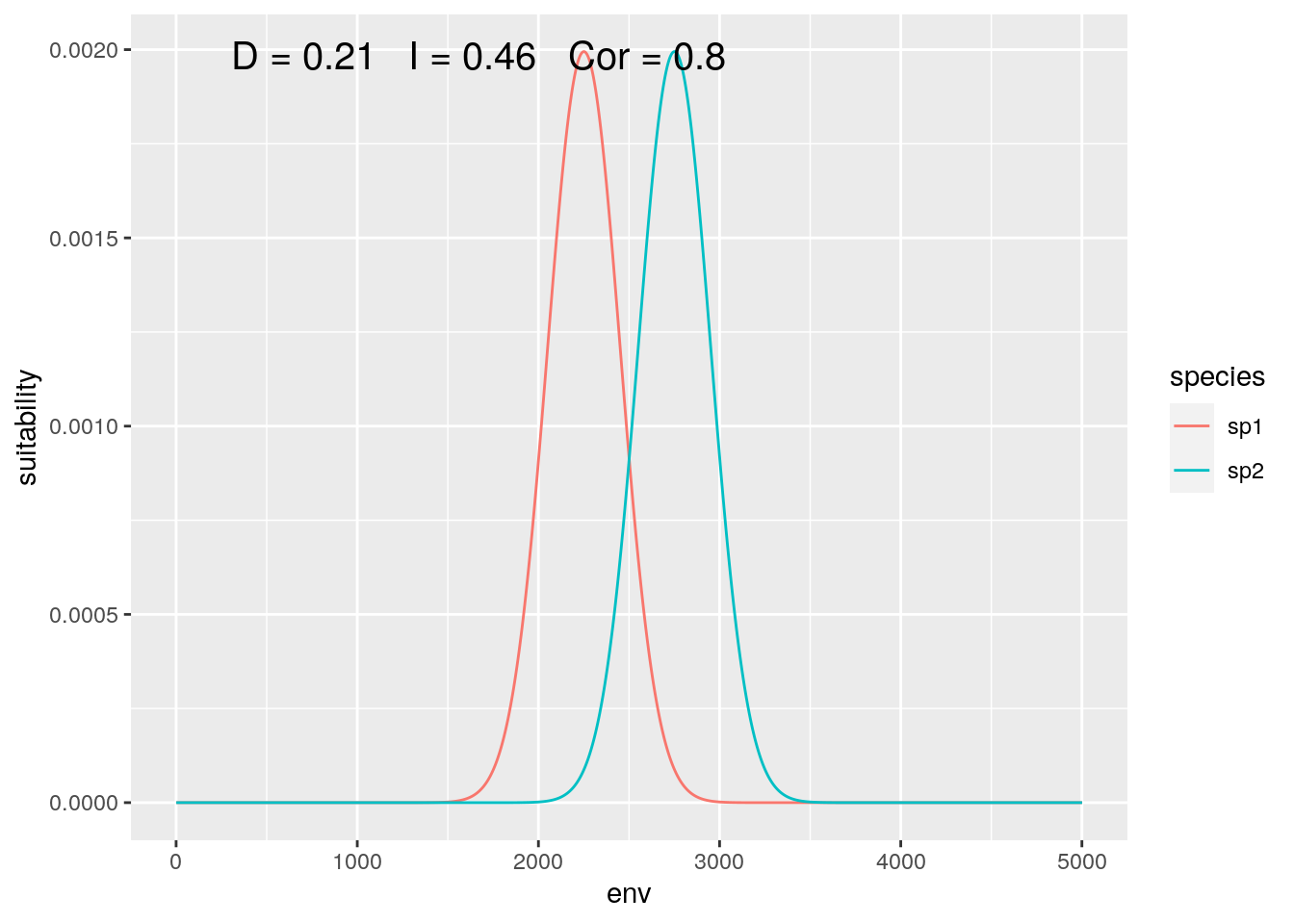

Figure 3: Global Analysis

At this scale, their response to the gradient appears to be highly correlated, while they have low niche overlap.

If we zoom in a bit, and ‘trim’ off the lowest and highest 1000 values on our gradient, we can emulate a ‘continental’ extent:

## ignore the lowest and highest 1000
## environmental values 
slice <- 1000:4000 

olaps(sp1[slice], sp2[slice])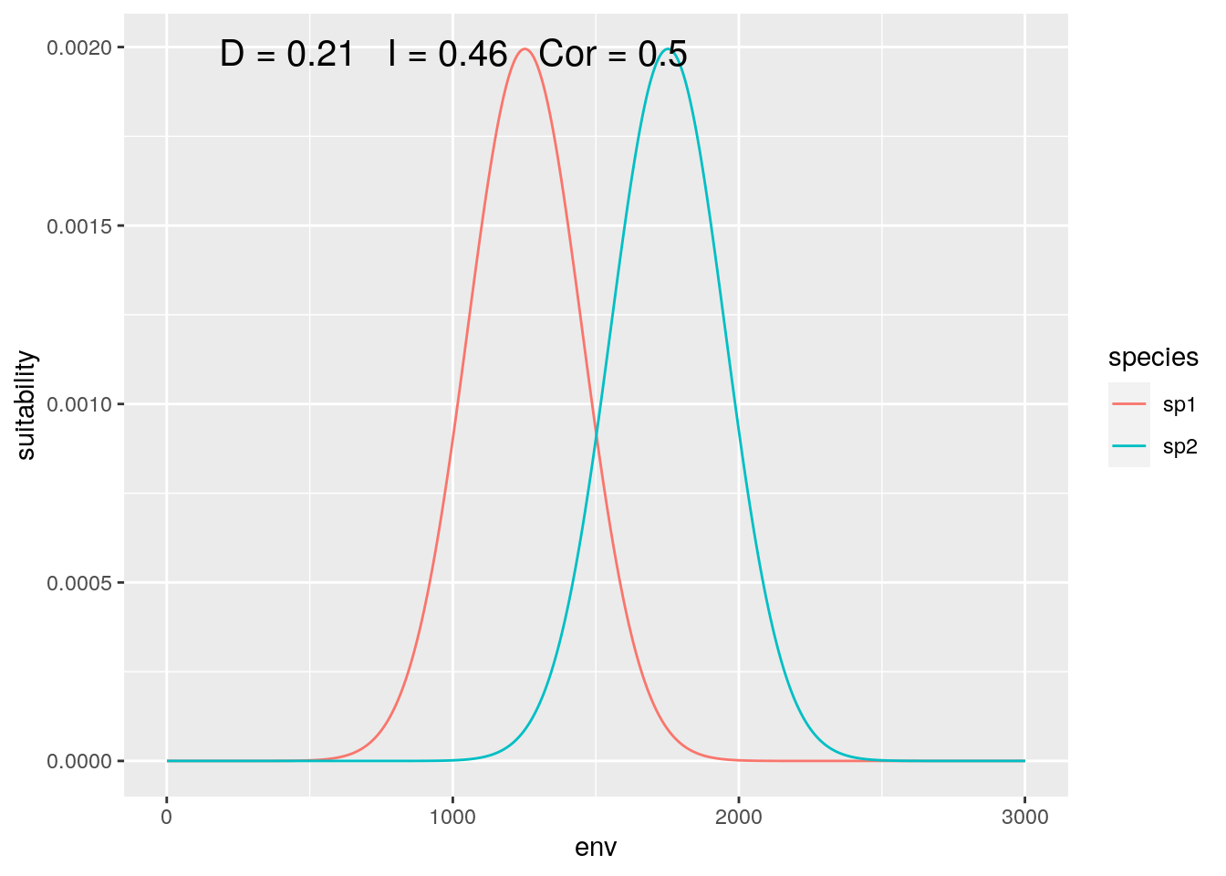

Figure 4: Continental Analysis

Correlation drops, but niche overlap remains identical. On reflection, this makes sense. Locations where neither species are present get no weight in the calculation of D, so dropping ‘empty’ gradient has no impact. On the other hand, those locations do contribute to inflating correlation.

Now what if we shift our focus, such that the distribution of our species is not equally represented:

slice <- 1000:2500 
olaps(sp1[slice], sp2[slice])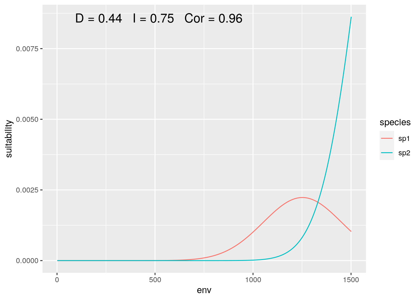

Figure 5: Regional Analysis

Correlation jumps up, as despite both species increase together over most of the sampled gradient. And with this particular slice, our niche overlap is twice the ‘true’ value when we consider the full gradient.

Finally, we can zoom in on the center of the gradient, where both species are equally represented (although with inverse responses):

slice <- 2000:3000
olaps(sp1[slice], sp2[slice])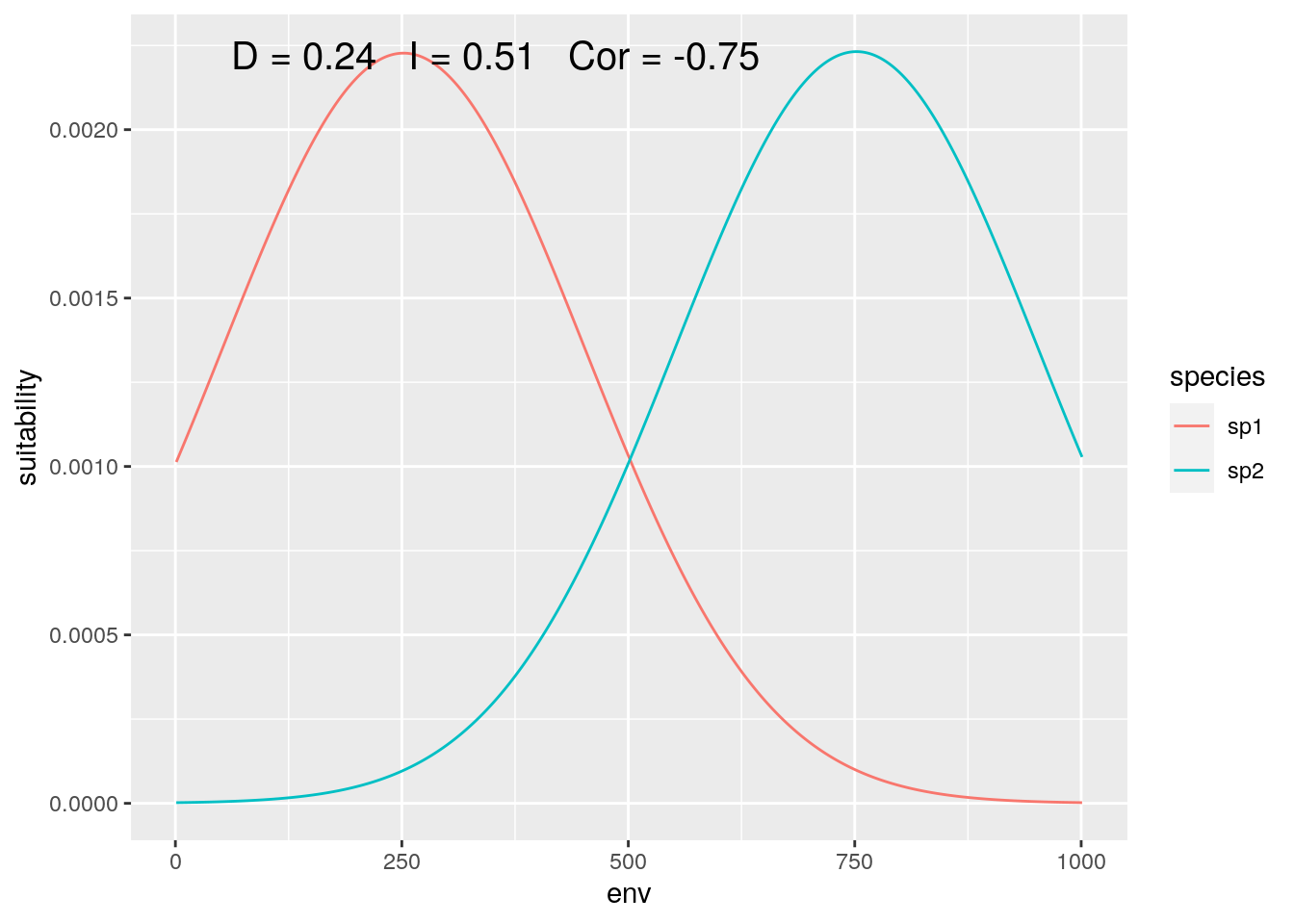

Figure 6: Contact Zone

Correlation drops again, accurately reflecting the inverse pattern. And D is back down close to the ‘true’ value. That’s ‘lucky’, as my toy species have perfectly symmetrical distributions, so sufficently large, symmetrical regions around the mid-point between the two of them will give reasonably accurate estimates.

Implications

Why does this matter? If you’re interested in comparing the environmental responses of two species, the results (correlation) can vary quite dramatically depending on the extent of your study.

On the other hand, Schoener’s D is robust to data that includes ‘too much’ of a gradient (i.e., extending beyond the region occupied by either species). But it can be sensitive to undersampling a gradient, where the relative occupancy of each species varies depending on how you set set your extent.

In other words, if you’re interested in the ‘underlying models’ that govern species’ comparative distributions along a gradient, you need to be very clear about the scope of the question, and how much of the environmental gradient you sample. But if you want to quantify niche overlap (or relative niche shift), then you want to include environments well beyond the regions actually occupied by your study organisms.

All of which is trivial to do when you get to create the species on the computer, and much trickier when you need to infer the details from museum records and climate rasters!