Introduction
This is an update of my previous ecospat
tutorial. Spatial analysis in R is shifting to
terra and sf as the primary packages, so I’ve translated my old,
raster-based tutorial to the new workflow. I also took this opportunity
to clean up and extend the original tutorial.
See the RSpatial tutorial for a
more detailed introduction/overview of using terra for GIS/spatial
analysis.
Note this analysis depends on the ecospat package, and as of 2023-07-28
ecospat doesn’t support the spatial objects produced by terra. There
are a couple of work-arounds in the code below to account for this. I’ll
update the code once ecospat is fully compatible with terra
UPDATE 2024-05-10 ecospat has now been updated to use the terra
package for spatial analysis. The code here has been updated to reflect
this. Thank you to Lin Lin at Yunan University for bringing this to my
attention!
The ecospat package (Cola et al. 2017) provides code to quantify and
compare the environmental and geographic niche of two species, or of the
same species in different contexts (e.g., in its native and invaded
ranges). The included vignette explains how to do such analyses.
However, the vignette assumes you already have a matrix of occurrence records, along with the climate data for each of those records. In our work, we typically have to construct those matrices from observation data (herbarium records, iNaturalist observations, etc) and climate rasters (e.g. Fick and Hijmans 2017). This short tutorial will walk through the steps necessary to do this.
Required Packages
In addition to ecospat, we’ll use terra (Hijmans 2023) to download
WorldClim (Fick and Hijmans 2017) rasters, and manipulate the spatial data;
rgbif (Chamberlain et al. 2021) to download GBIF records, geodata
(Hijmans et al. 2023) to get a world basemap for plots, and ade4
(Thioulouse et al. 2018) to perform the principal components analysis of the
climate data.
library(ecospat)
library(terra)
library(rgbif)
library(geodata)
library(ade4)
Getting Data
GBIF Occurrence Data
We’ll start by sourcing our data. For observations, let’s take a look at
Purple Loosestrife, a wetland species that is native to Europe, and
invasive in North America. For actual research work, I normally download
the files directly from GBIF, and examine them carefully to check for
errors or missing data. For this demo we’ll use the rgbif package to
download the data directly into R, and we’ll assume there are no problems
with the data that need to be corrected.
lsGBIF <- occ_search(scientificName = "Lythrum salicaria",
                    limit = 10000,
                    basisOfRecord = "Preserved_Specimen",
                    hasCoordinate = TRUE,
                    fields = c("decimalLatitude",
                               "decimalLongitude", "year",
                               "country", "countryCode"))

save(lsGBIF, file = "../data/2021-07-29-ls-gbif-recs.Rda")
This returned an object with 7969 records. I saved that locally, so that I’m not making GBIF search their database everytime I work on this demo.
load("../data/2021-07-29-ls-gbif-recs.Rda")
lsOccs <- lsGBIF$data
lsGBIF$data is the table with the actual records in it. That’s what we’ll
be working with. The other components of lsGBIF are metadata related to
the original GBIF search. That’s useful to have, but not needed for the
rest of this example.
Next, we tell R which columns are the coordinates, which allows us to map
the observations. This also converts our observation matrix to a
SpatVector object.
The crs argument here tells R that our points are in lat/lon
(unprojected) coordinates. If all of your data use lat/lon, you don’t need
to specify this, but it’s important if you need to reproject your data, or
combine data with different projections.
lsOccs <- vect(lsOccs, geom = c("decimalLongitude",
                                "decimalLatitude"),
               crs = "+proj=longlat +datum=WGS84")
Basemap
We’ll also need a world map to use in our plots. the world function from
the geodata package will download one for us. The first time you call
this function in a directory, it downloads the data from the internet,
and saves it locally according to the path argument. Subsequent calls
will load your local copy of the data, to speed things up.
In this case I’ve set the path argument to store the downloaded files in
a location that is convenient for me. You can set this to anything you
like, or leave it out to use the current R working directory.
wrld <- world(path = "../data/maps/")This is a relatively low resolution map of the continents. For higher
resolution maps, see the gadm function.
Now we can plot our data. Note that we set the margins (via mar) inside
the plot call, not via the par function used in most base R plots.
plot(wrld, border = "gray80", mar = c(0, 0, 0, 0))
points(lsOccs, col = 2, cex = 0.3)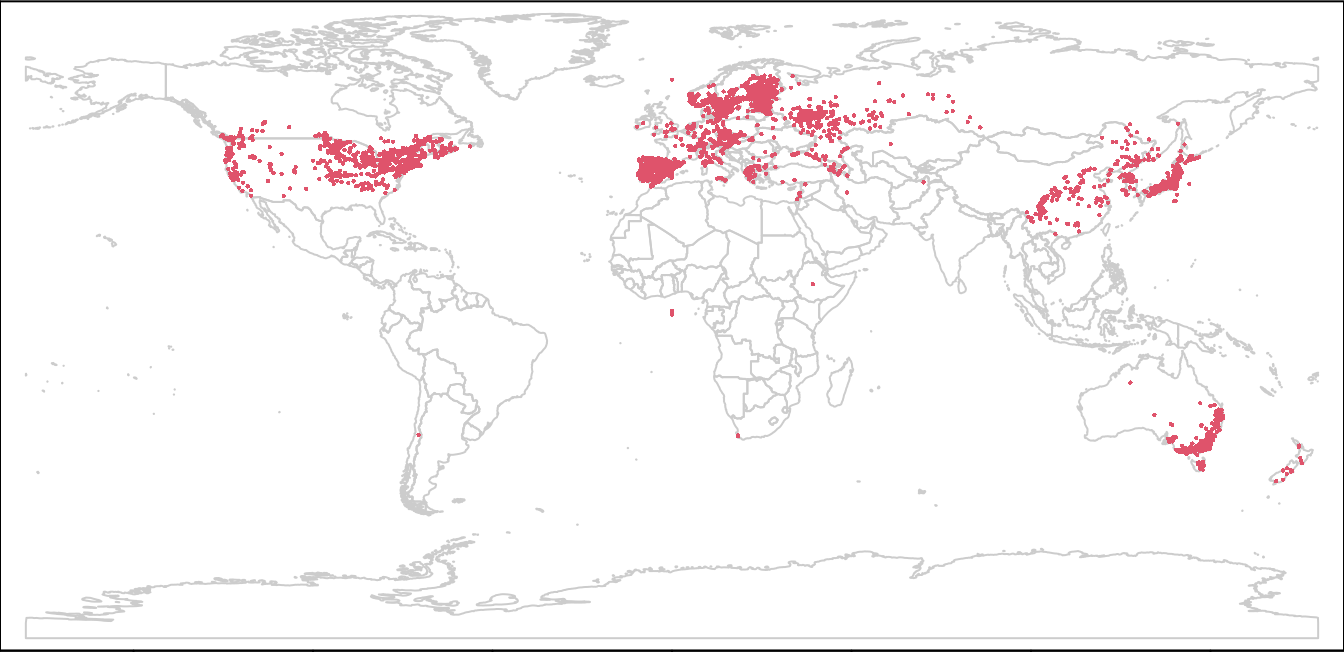
Climate Data
To get our climate data, we can use geodata’s worldclim_* functions.
I’m using the coarsest resolution (10 minutes) to speed things up for this
demonstration. The path argument works the same was as for world,
storing a local copy of the files. In this instance we’ll use
worldclim_global to get the bioclim variables for the world all at once:
wclim <- worldclim_global(var = "bio", res = 10,
                          path = "../data/")
We can take a look at one layer:
plot(wclim$wc2.1_10m_bio_1, main = "bio1",
     mar = c(0.1, 0.1, 2, 4), legend = TRUE,
     axes = FALSE)
par(mar = c(0.1, 0.1, 2, 4))
box()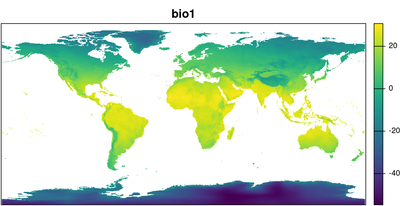
Sampling Bias
One of the challenges we deal with with herbarium data is that observations tend to be clustered together in non-random ways. Sites near universities, museums, or in well-used field stations will have more records than more remote locations. We can’t completely account for this bias, but we can reduce it by spatial thinning. This is the process of randomly selecting a small number (often just one) of records for each grid cell in our analysis. The result is that those highly-sampled locations will be represented by a single record, meaning they will have a less exaggerated influence on the results.
We will need the full set of records below, so I’ll make a copy of the
un-thinned data named lsOccsAll.
lsOccsAll <- lsOccs ## keep this for later

## select one record per cell:
lsOccs <- spatSample(lsOccs, size = 1, strata = wclim)
Linking Climate Data to Species Observations
Next, we need to extract the environmental values from the climate rasters for each of our observation records:
lsOccs <- cbind(lsOccs, extract(wclim, lsOccs))In the process of extracting wclim values for our observations, we
usually end up with a few missing values. This is a consequence of
mismatches between the observation coordinates and the climate rasters. In
some cases, the observations are placed off the coast in the ocean, or in
another area where there is no climate data available. We need to exclude
these missing values from our analysis.
lsOccs <- lsOccs[complete.cases(data.frame(lsOccs)), ]Splitting Records into Native and Introduced Ranges
At this point, all the data we need for the Niche Quantification analysis
is in lsOccs and wclim. We need to split this data into native and
invasive regions for our comparison. We’ll restrict ourselves to the
northern hemisphere, and consider all records from Eurasia as native, and
all records from North America as invasive.
We can use GADM to download maps of the continents, and use this to select
subsets of the datasets. I will select the country-level borders (level = 0) and low resolution (resolution = 2). For ‘real’ analyses you should
use high resolution (resolution = 1).
To speed up analyses further down, I’m just going to download Canada, USA, and Mexico for my “North America” map.
nAmCountries <- c("CAN", "MEX", "USA")
nAm <- gadm(nAmCountries, level = 0,
            path = "../data/maps/",
            resolution = 2)

## select Europe OR Asia:
eurasiaCountries <- country_codes("Asia|Europe")
eur <- gadm(eurasiaCountries$ISO3, level = 0,
            path = "../data/maps/",
            resolution = 2)

lsNA <- lsOccs[nAm]
lsEA <- lsOccs[eur]

plot(wrld, axes = FALSE, xlim = c(-140, 150),
     ylim = c(10, 80), mar = c(0, 0, 0, 0))
points(lsNA, col = 'red', cex = 0.5)
points(lsEA, col = 'darkgreen', cex = 0.5)
par(mar = c(0,0,0,0))
box()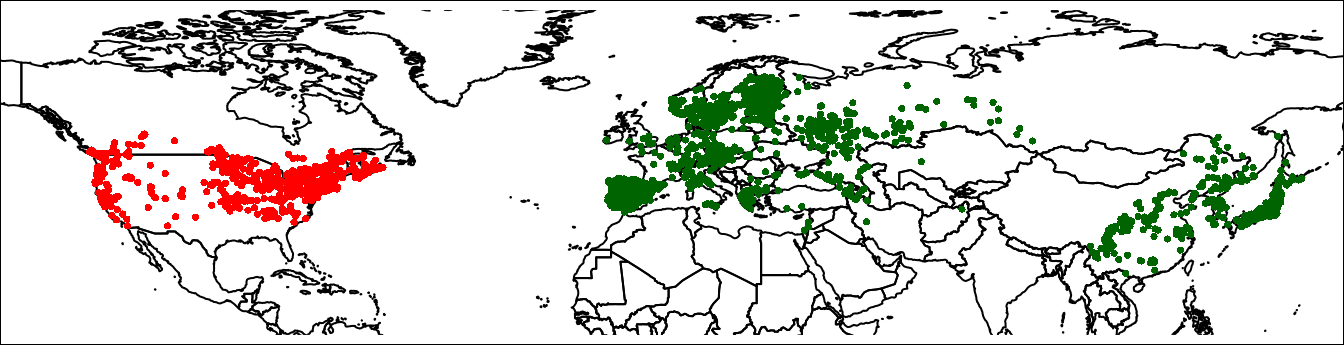
Note that this code will generate some warnings, “this file does not
exist”. There are a few countries listed in the country_codes database
that don’t have corresonding maps in the GADM repository (e.g. Hong Kong).
We’ll ignore this for now.
For the Niche Quantification, we need to have a matrix with the background
environment present in the native and invasive ranges, as well as the
complete global environmental including the combined extent of the native
and introduced environments. After cropping the data, we use values
to convert the raster to a dataframe.
## Crop Climate Layers:
naEnvR <- mask(wclim, nAm)
## |---------|---------|---------|---------|========================================= eaEnvR <- mask(wclim, eur)## |---------|---------|---------|---------|========================================= globalEnvR <- mask(wclim, rbind(nAm, eur))## |---------|---------|---------|---------|========================================= ## Extract values to matrix:
naEnvM <- values(naEnvR)
eaEnvM <- values(eaEnvR)
globalEnvM <- values(globalEnvR)
## Clean out missing values:
naEnvM <- naEnvM[complete.cases(naEnvM), ]
eaEnvM <- eaEnvM[complete.cases(eaEnvM), ]
globalEnvM <- globalEnvM[complete.cases(globalEnvM), ]Note that for the geographic projection below, it is essential that the
globalEnvM be constructed directly from the globalEnvR rasters. If you
try to combine naEnvM and eaEnvM to make globalEnvM it will end up
scrambling the values in the geographic projection. If you don’t do a
geographic projection it doesn’t matter.
Niche Quantification
PCA
The Niche Quantification analysis starts with a Principal Components Analysis of the environmental data. The actual ordination uses the global data, with the observation records and the native and invasive background environment treated as supplemental rows.
pca.clim <- dudi.pca(globalEnvM, center = TRUE,
                    scale = TRUE, scannf = FALSE, nf = 2)
global.scores <- pca.clim$li

nativeLS.scores <-
  suprow(pca.clim,
         data.frame(lsEA)[, colnames(globalEnvM)])$li
invasiveLS.scores <-
  suprow(pca.clim,
         data.frame(lsNA)[, colnames(globalEnvM)])$li

nativeEnv.scores <- suprow(pca.clim, naEnvM)$li
invasiveEnv.scores <- suprow(pca.clim, eaEnvM)$li
Let’s break that down. dudi.pca does a PCA analysis on globalEnvM,
which is a matrix of all the environmental variables over the entire study
area. We use that to create a two-dimensional summary of the total
environmental variability.
Next, we map our observation data (lsEA and lsNA) into that
2-dimensional ordination, using the suprow function. lsEA and lsNA
are SpatialPointsDataFrame objects. Sometimes you can treat them as if
they were data.frames, but other times you need to explicity convert them.
This is one of those times, hence I’ve wrapped them in data.frame().
Recall that lsEA and lsNA have more columns than the environmental
matrix: they also include year, countryCode, country. We only want to
include the environmental variables when you project the observations into
the ordination. To make sure that we use the same variables as in the
original ordination of globalEnvM, in the same order, I select the
columns explicitly to match that object:
data.frame(lsEA)[, colnames(globalEnvM)]The output of dudi.pca and suprow includes a lot of information that we
aren’t using here. We only need the li element, so I’ve selected that
from each of the function outputs.
Occurrence Density Grids
Finally we’re ready to do the Niche Quantification/Comparisons. We’ll use the PCA scores for the global environment, the native and invasive environments, and the native and invasive occurrence records.
nativeGrid <- ecospat.grid.clim.dyn(global.scores,
                                   nativeEnv.scores,
                                   nativeLS.scores)

invasiveGrid <- ecospat.grid.clim.dyn(global.scores,
                                   invasiveEnv.scores,
                                   invasiveLS.scores)

ecospat.plot.niche.dyn(nativeGrid, invasiveGrid,
quant = 0.05) 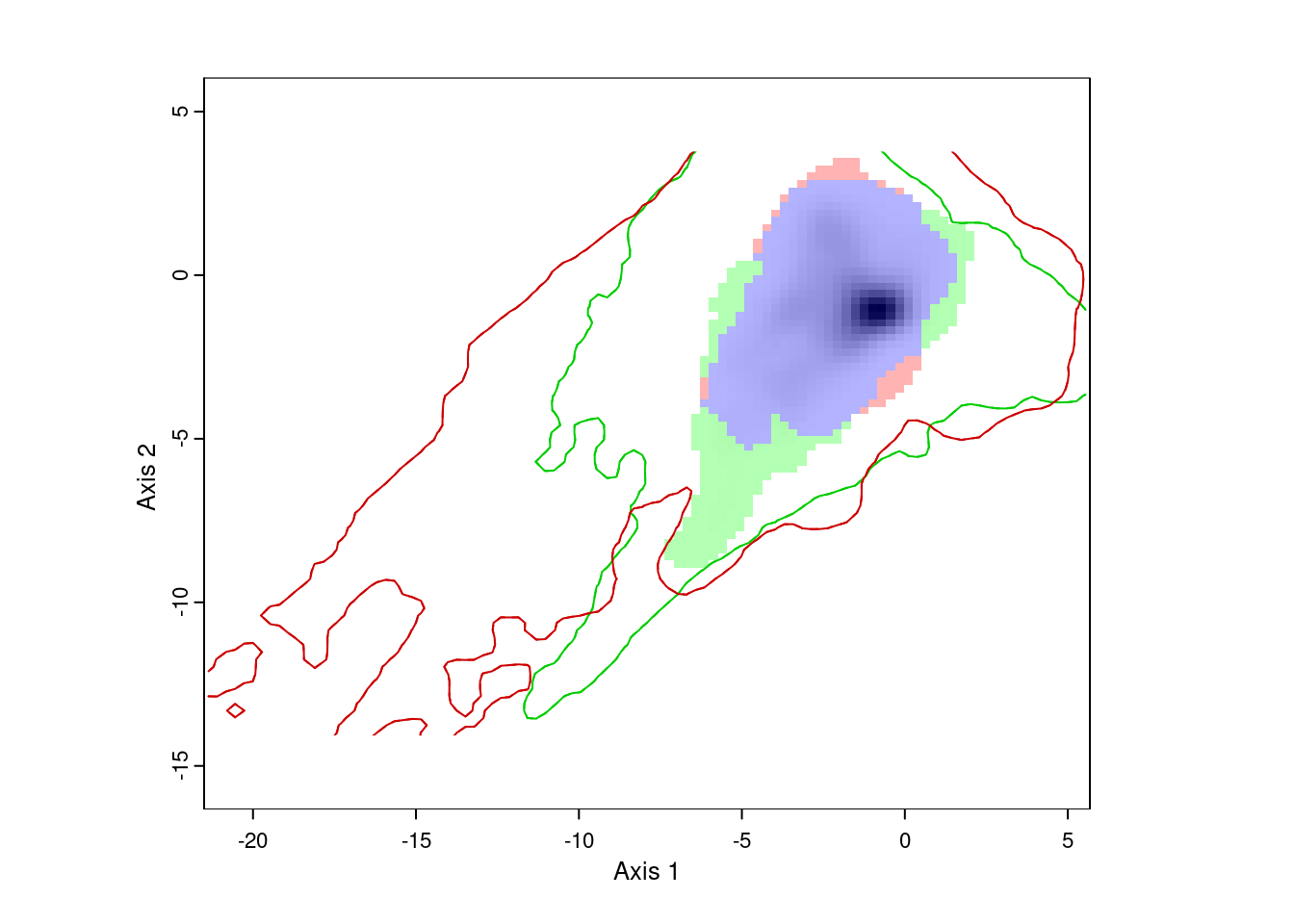
The resulting plot shows us the environmental conditions present in Eurasia (inside the green line) and North America (inside the red line). The green area represents environments occupied by Lythrum salicaria in Eurasia, but not in North America, the red area shows environments occupied in North America and not Eurasia, and the blue area shows environments occupied in both ranges. We can also see that there are a few areas in Eurasia with environments not present in North America, and vice versa. However, for the most part, Lythrum salicara doesn’t occur in this environments.
To get the index values we use ecospat.niche.dyn.index:
indexVals <- ecospat.niche.dyn.index(nativeGrid,
                                     invasiveGrid)
indexVals$dynamic.index.w
## expansion stability unfilling
## 0.00598794 0.99401206 0.02349507Projecting Climate Space to Geographic Space
We can take these results and project them onto a geographic map. This will show us which areas of the native and invasive range of Lythrum salicaria fall into each of the three categories.
Note that the function ecospat.niche.dynIndexProjGeo doesn’t yet handle
the SpatRaster objects created by the terra package, so we have to
convert it to a raster’s stack when we call it. For convenience and
consistency with the rest of the code, I convert the results back to a
SpatRaster.
geoProj <-
  ecospat.niche.dynIndexProjGeo(nativeGrid,
                                invasiveGrid,
                                env = globalEnvR)

plot(geoProj, legend = FALSE,
     col = c("grey", "green", "red", "blue"),
     ylim = c(20, 80), axes = FALSE, mar = c(0, 0, 0, 0))
points(lsEA, col = 'darkgreen',
       cex = 0.25, pch = 23, bg = "white")
points(lsNA, col = 'darkred',
       cex = 0.25, pch = 23, bg = "white")
par(mar = c(0,0,0,0))
box()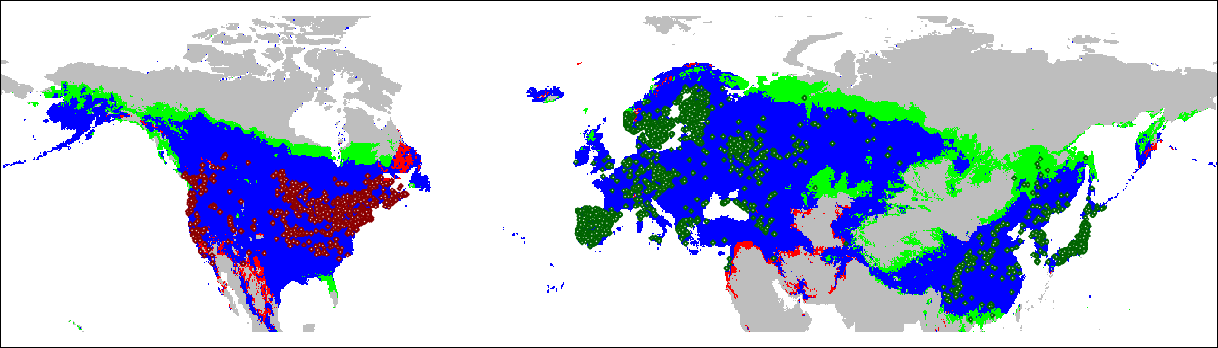
Geographic Comparisons
You can also apply this analysis to geographic locations, instead of environmental conditions. This won’t make much sense for native vs invaded range comparisons, but it could be useful for comparing different species within the same area.
To demonstrate, let’s compare the distribution of Lythrum salicaria in North America before and after 1950. In this case, I need to go back to the original occurrence data, since I need the thin the records before and after 1950 separately. Otherwise, we won’t accurately capture the locations where Lythrum salicaria was collected in both time periods.
We use geographic coordinates here, so no need for a PCA. We do need to
generate the ‘background’ coordinates. I’ll use expand.grid to create the
locations for this. I’ve broken up the NA extent into 500 x 500 grids.
lsNA_All <- lsOccsAll[nAm]

lsNAearly <- subset(lsNA_All, lsNA$year <= 1950)
## thin records:
lsNAearly <- spatSample(lsNAearly, size = 1, strata = wclim)

lsNAlate <- subset(lsNA_All, lsNA$year > 1950)
## thin records:
lsNAlate <- spatSample(lsNAlate, size = 1, strata = wclim)

geoGrid <- expand.grid(longitude =
                        seq(-160, -40, length.out = 500),
                      latitude =
                        seq(20, 90, length.out = 500))

earlyGeoGrid <- ecospat.grid.clim.dyn(geoGrid, geoGrid,
                                     crds(lsNAearly))

lateGeoGrid <- ecospat.grid.clim.dyn(geoGrid, geoGrid,
                                    crds(lsNAlate))

ecospat.plot.niche.dyn(earlyGeoGrid, lateGeoGrid, quant = 0)
plot(nAm, add = TRUE)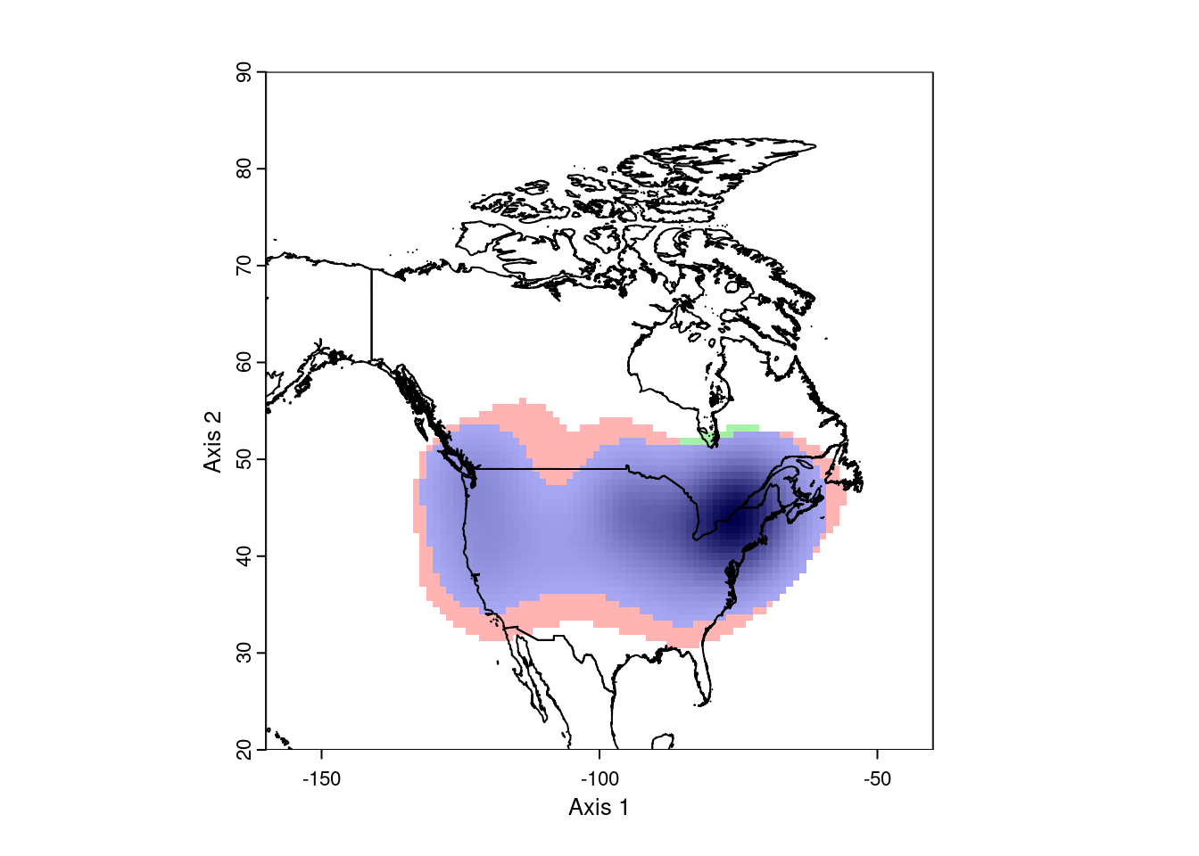
This looks pretty good. However, ecospat uses a kernel density formula to
model the occurence distributions. As a consequence, it projects out into
the ocean, which isn’t very realistic. To correct this, we need to mask the
analysis to the continental land mass. This requires we have a vector map
of the desired area.
earlyGeoGrid <- ecospat.grid.clim.dyn(geoGrid, geoGrid,
                                     crds(lsNAearly),
                                     geomask = nAm)

lateGeoGrid <- ecospat.grid.clim.dyn(geoGrid, geoGrid,
                                    crds(lsNAlate),
                                    geomask = nAm)

ecospat.plot.niche.dyn(earlyGeoGrid, lateGeoGrid, quant = 0)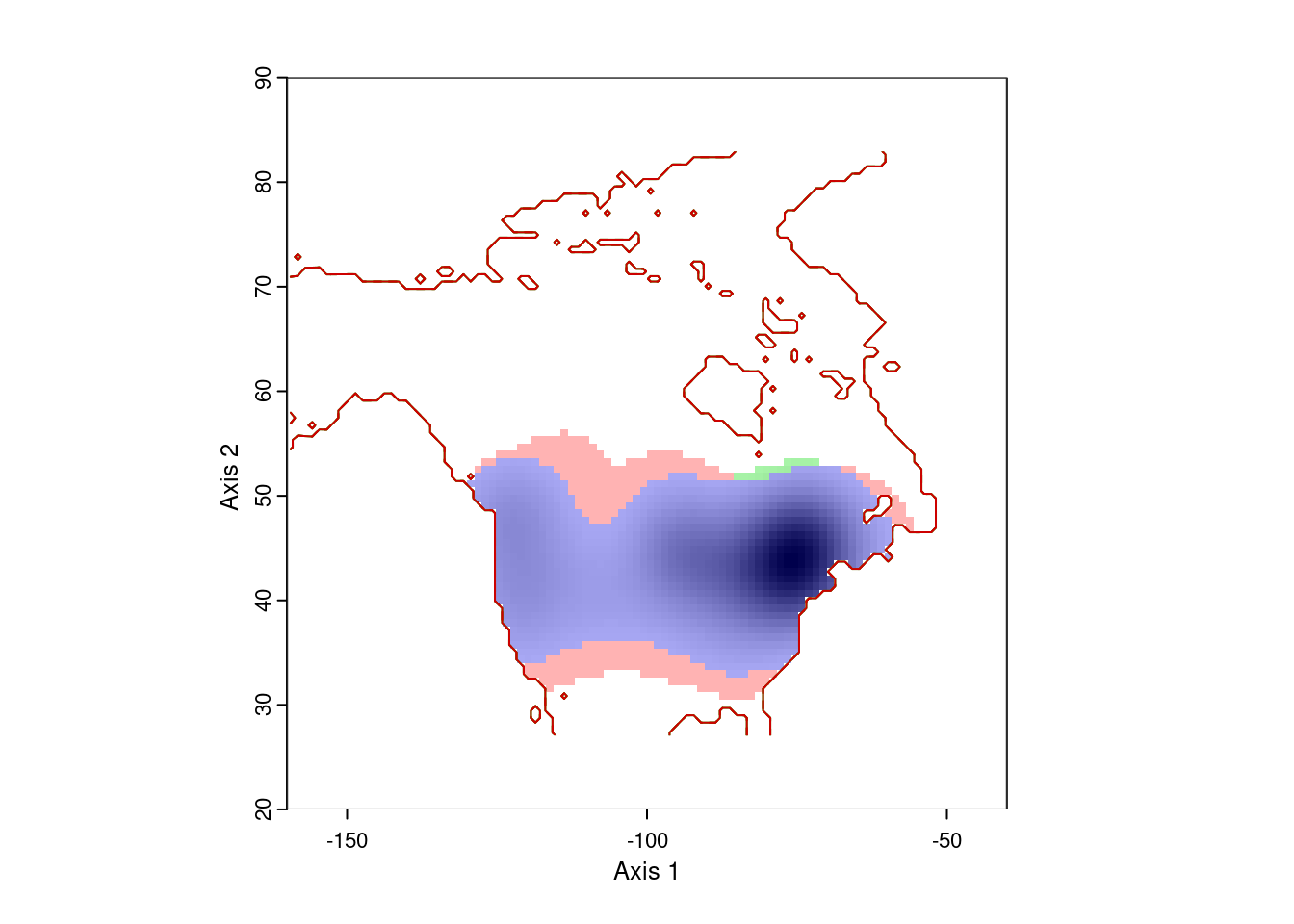
That gives more reasonable results. The blue area is the range occupied by Lythrum salicara prior to 1950, and the red area is the range it expanded into after that year. The small green areas are regions where it hasn’t been collected since 1950.
Note that this visualization is weighted by the density of points, so there might be a few pre-1950 records in the red area, or a few post-1950 records in the red area. That’s expected.
Summary
This is a fairly quick overview of this workflow. You’ll almost certainly want to consider thinning your observations, among other data cleaning procedures. I’ve also set the study extent very crudely. That might be appropriate for very large scale (global) studies. But you’ll usually want to think a bit more carefully about how you set your extent. The way you process your data will also differ depending on your context.
References
Chamberlain, Scott, Vijay Barve, Dan Mcglinn, Damiano Oldoni, Peter Desmet, Laurens Geffert, and Karthik Ram. 2021. “Rgbif: Interface to the Global Biodiversity Information Facility API.” Manual. https://CRAN.R-project.org/package=rgbif.
Cola, Valeria Di, Olivier Broennimann, Blaise Petitpierre, Frank T. Breiner, Manuela D’Amen, Christophe Randin, Robin Engler, et al. 2017. “Ecospat: An R Package to Support Spatial Analyses and Modeling of Species Niches and Distributions.” Ecography 40 (6): 774–87. https://doi.org/10.1111/ecog.02671.
Fick, Stephen E., and Robert J. Hijmans. 2017. “WorldClim 2: New 1-Km Spatial Resolution Climate Surfaces for Global Land Areas.” International Journal of Climatology 37 (12): 4302–15. https://doi.org/10.1002/joc.5086.
Hijmans, Robert J. 2023. “Terra: Spatial Data Analysis.” Manual. https://CRAN.R-project.org/package=terra.
Hijmans, Robert J., Márcia Barbosa, Aniruddha Ghosh, and Alex Mandel. 2023. “Geodata: Download Geographic Data.” Manual. https://CRAN.R-project.org/package=geodata.
Thioulouse, Jean, Stéphane Dray, Anne-Béatrice Dufour, Aurélie Siberchicot, Thibaut Jombart, and Sandrine Pavoine. 2018. Multivariate Analysis of Ecological Data with Ade4. New York, NY: Springer New York. https://doi.org/10.1007/978-1-4939-8850-1.