Identifying Non-Analogous Climate Conditions
A major concern when projecting species distribution models to new contexts (e.g., invaded ranges, or future climates) is establishing whether (and where) the environments in the new context are analogous to those in the training region (see my notes). A common approach is to compare each variable in isolation, and construct a “Multivariate Environmental Similarity Surface”, or MESS (Elith et al., 2010). Areas in the new context that are outside the range of any variable from the training context will have values below 0, with lower values indicating greater departures.
However, the MESS approach does not account for correlations among variables. Perhaps the native range of a species includes areas with hot, wet, summers, but not hot dry regions. The MESS analysis would consider conditions ‘analogous’ as long as they were within the temperature range and precipitation range of the training region. This could result in novel environmental combinations being incorrectly identified as analogous climate:
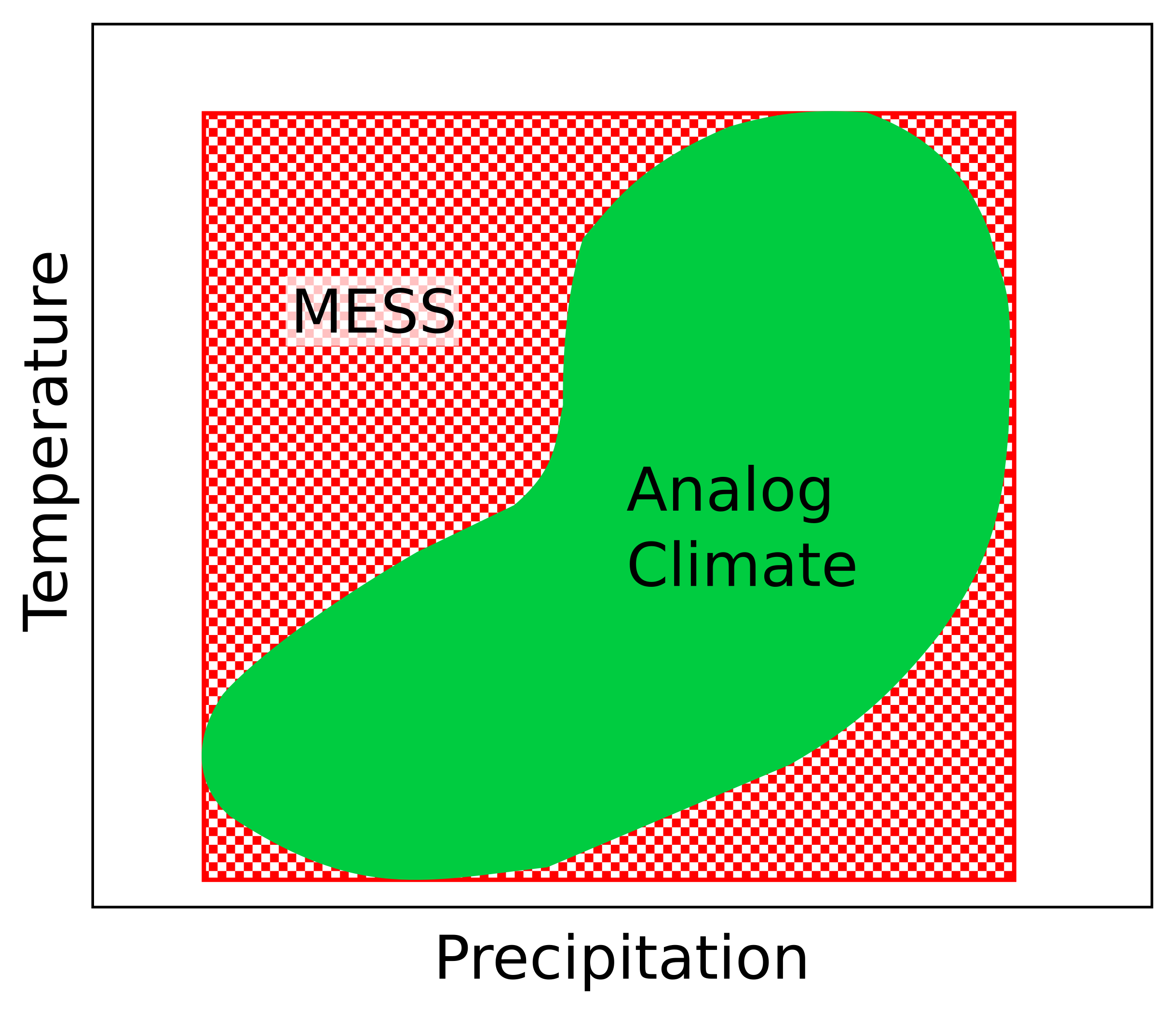
Visualization of MESS analysis. The green area indicates the reference climate conditions, and the red square shows the climate space MESS will identify as ‘analog’.
Note particularly the upper left corner. This is well outside the range of conditions in the training region (the green area), but by considering each variable separately, MESS will treat this region as if it were analogous.
Extrapolation Detection
Despite the name, MESS is only just barely multivariate: it evaluates
multiple variables, but each one is considered in isolation. Extrapolation
Detection (Mesgaran et al., 2014), or exDet, provides a more sophisticated
approach, based on the Mahalanobis distance. This is a common multivariate
distance measure, designed to account for covariation among variables. In
this context, our analysis will include the following steps:
- Calculate the Mahalanobis distance for every cell in the training region
- Scale the distances by dividing by the maximum distance, such that they range between 0 and 1
- Calculate the Mahalanobis distance for every cell in the novel region/time period, again dividing by the maximum distance from the training (not the new) region.
This will produce a raster map with cell values ranging from 0 to infinity,
which serves as the Novelty Index. Mesgaran et al. (2014) refer to it as NT2,
to distinguish it from the MESS index which they call NT1. Cells with NT2
values less than 1 are within the range of conditions present in the
training range; cells with NT2 > 1 are outside that range, with higher
values indicating greater departure:
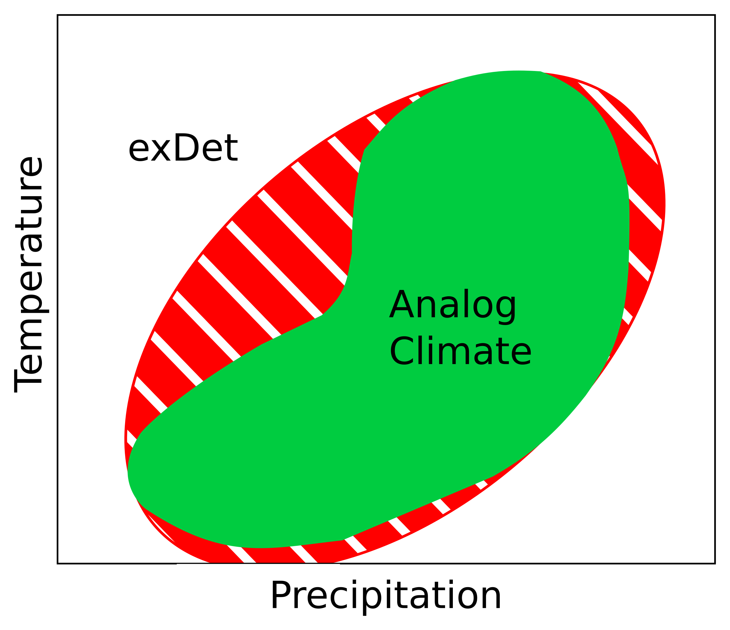
Visualization of exDet analysis. The green area indicates the reference climate conditions, and the red ellipse shows the climate space exDet will identify as ‘analog’.
The result more closely captures the (co)variation in conditions present in the training area.
exDet in R
There is an R package that calculates exDet:
ntbox. However, it is still using the
raster-based workflow, which is now obsolete. Luckily, calculating
Mahalanobis distances only requires a few lines of code, so we can do it
ourselves.
For this example, I’ll use the Lythrum salicaria data from my previous tutorials, but updated to use the new terra workflow.
Data
I use the same GBIF records previously downloaded in my Ecospat with Terra tutorial.
library(terra)
library(geodata)
library(rgbif) ## not actually necessary, used to download
               ## the occurrence data

library(usdm) ## for vif collinearity test below

load("../data/2021-07-29-ls-gbif-recs.Rda")
lsOccs <- lsGBIF$data

## convert to a spatial vector:
lsOccs <- vect(lsOccs, geom = c("decimalLongitude",
                                "decimalLatitude"),
               crs = "+proj=longlat +datum=WGS84")

wrld <- world(path = "../data/maps/")

wclim <- worldclim_global(var = "bio", res = 10,
                          path = "../data/")

## North America basemap:
nAmCountries <- c("CAN", "MEX", "USA")
nAm <- gadm(nAmCountries, level = 0,
            path = "../data/maps/",
            resolution = 2)

## Eurasia basemap:
eurasiaCountries <- country_codes("Asia|Europe")

## remove missing countries:
eurasiaCountries <-
  eurasiaCountries[!eurasiaCountries$ISO3 %in%
                    c("HKG", "MAC", "XNC"),]
eur <- gadm(eurasiaCountries$ISO3, level = 0,
            path = "../data/maps/",
            resolution = 2)

## subset occurrences
lsNA <- lsOccs[nAm]
lsEA <- lsOccs[eur]
Training Region
There are a number of considerations when deciding on the region to use to train our model. For this example, I’ll just use a 500km buffer around occurrences in the native range.
Now we have all the data we need for the analysis:
train <- buffer(lsEA, width = 500000)
train <- aggregate(train)

plot(wrld, mar = c(1.5, 1.5, 0.5, 0.5))
plot(train, col = '#00FF0080', add = TRUE)
plot(lsEA, add = TRUE, cex = 0.5)
plot(lsNA, add = TRUE, cex = 0.5, col = 'blue')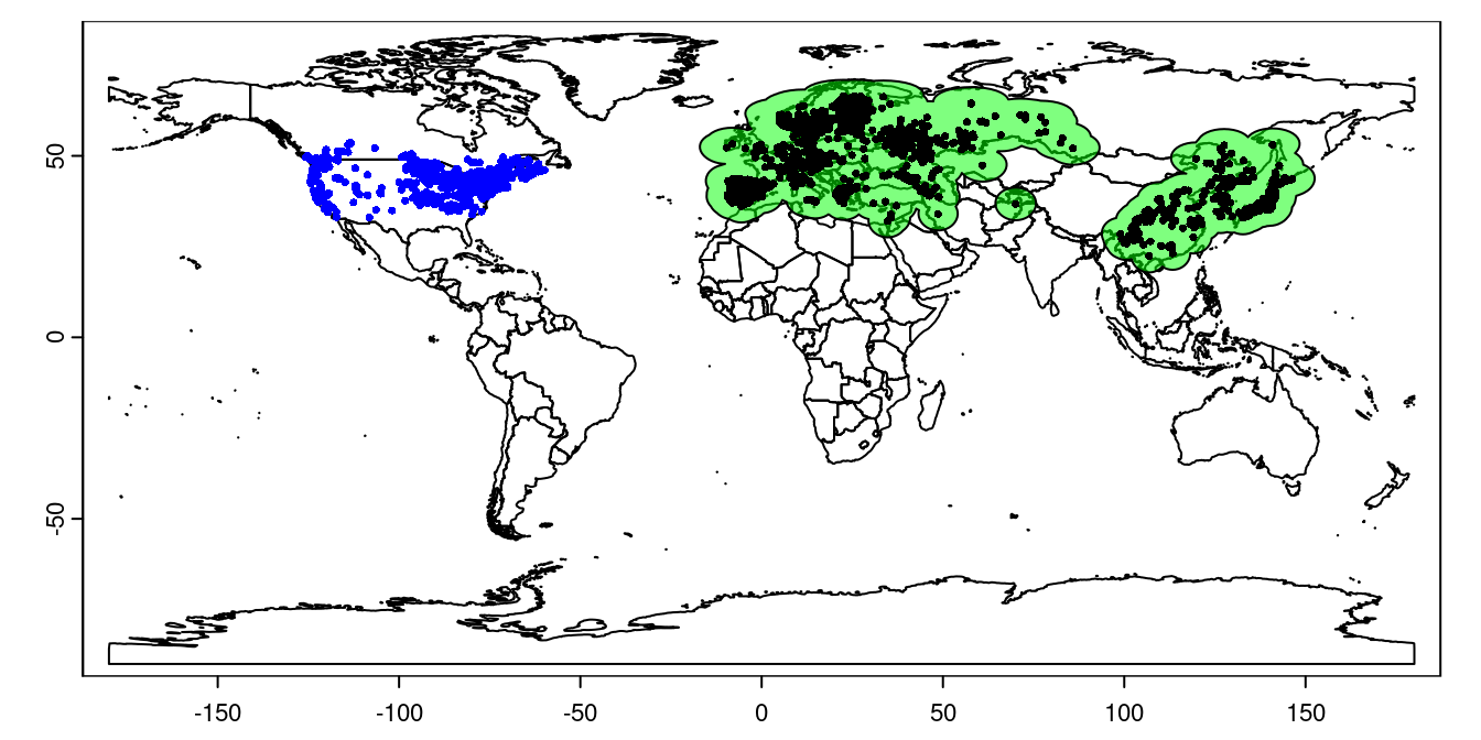
Figure 1: Lythrum salicaria distribution. Green shading shows the training region, black points are occurrences in the native range, and blue points are occurrences in the invaded range.
Note that the training region extends into the ocean, but the underlying worldclim data doesn’t, so we don’t need to worry about cleaning this up.
Mahalanobis Distance
Now we can calculate the NT2 index. We start by clipping the climate data to our training and projection regions, and then selecting a set of variables that aren’t highly collinear (in the training region):
trainWC <- mask(wclim, train)##
|---------|---------|---------|---------|
=========================================
trainVal <- values(trainWC)

naWC <- mask(wclim, nAm)
##
|---------|---------|---------|---------|
=========================================
naVal <- values(naWC)

## screen out collinear variables:
vifSel <- vifstep(data.frame(trainVal), th = 5,
                  size = 20000)

VARS <- vifSel@results$Variables
VARS contains a list of non-collinear variables. For a real analysis you
probably should be more deliberate in selecting which variables to retain,
in order to consider both their biological interest and statistical
properties.
trainMeans <- colMeans(trainVal[, VARS], na.rm = TRUE)
trainVar <- var(trainVal[, VARS], na.rm = TRUE)
trainMah <- mahalanobis(trainVal[, VARS], trainMeans,
                        trainVar, na.rm = TRUE)
trainMah now contains the Mahalanobis distance from each cell in the
training region to the climate centroid of the training region. ‘0’ means
the point is in the center of the climate space. By the nature of the
Mahalanobis distance, this value accounts for covariation among our climate
variables.
As a quick check, let’s take a look at the Mahalanobis distances for the training region:
hist(trainMah, main = "Mahalanobis Distances in Eurasia",
     xlab = "Distance")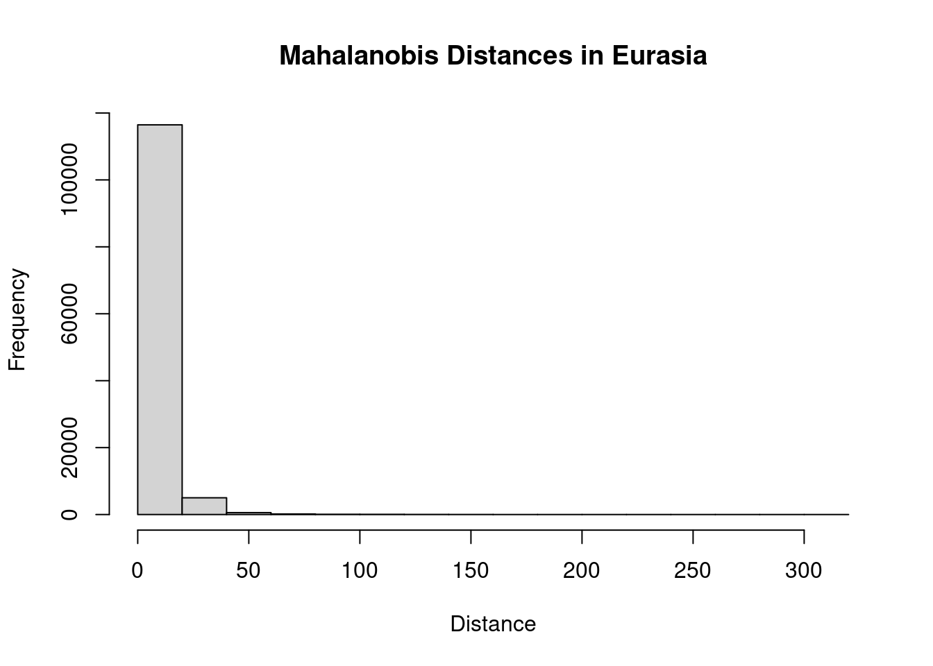
That’s a bit odd. We have a small number of outliers with very high distances. I think this is likely a consequence of idiosyncracies in our climate rasters: an artifact of the analysis rather than a biologically meaningful value. To clean this up, I’ll identify values above the 95th percentile as outliers and remove them. Then we can proceed with calculating the distances for the invaded range.
thresh <- quantile(trainMah, probs = 0.95, na.rm = TRUE)
trainMah[which(trainMah > thresh)] <- NA
hist(trainMah, main = "Trimmed Mahalanobis Distances in Eurasia",
     xlab = "Distance")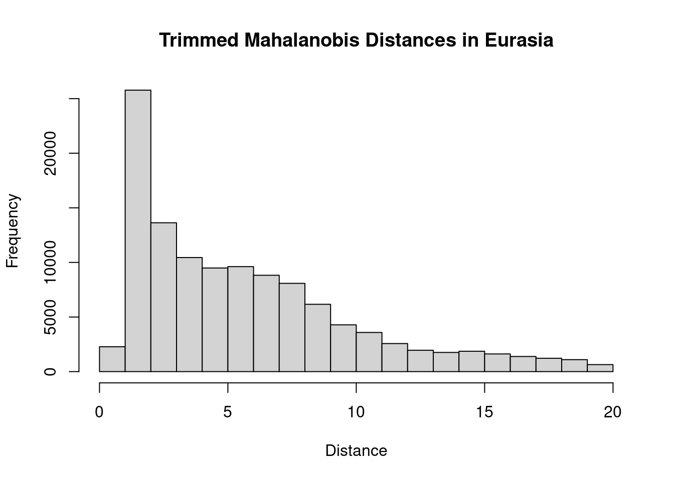
That looks better. Moving on, we can now calculate NT2, which is the Mahalanobis distance divided by the maximum Mahalanobis distance in the training range:
maxMah <- max(trainMah, na.rm = TRUE)
trainMah <- trainMah/maxMah
trainMahR <- trainWC[[1]]
values(trainMahR) <- trainMah

naMah <- mahalanobis(naVal[, VARS],
                     trainMeans, trainVar, na.rm = TRUE)
naMah <- naMah/maxMah

## Create a new raster map for North America:
naMahR <- naWC[[1]]

## set the values to our Mahalanobis distances:
values(naMahR) <- naMah
Now we have a raster map with the NT2 index values for each cell in the training and invaded ranges. Values between 0 and 1 are within the training range. We can visualize that directly:
COLS <- c("green", "lightgreen", "aquamarine", "blue",
           "orange", "brown", "red")

BREAKS = c(0, 0.25, 0.5, 1, 2, 4, 8, 16)

plot(trainMahR, breaks = BREAKS, col = COLS,
     mar = c(2, 2, 1, 5))
plot(naMahR, breaks = BREAKS, col = COLS, add = TRUE, legend
     = FALSE)
plot(wrld, border = 'lightgrey', add = TRUE, lwd = 0.5)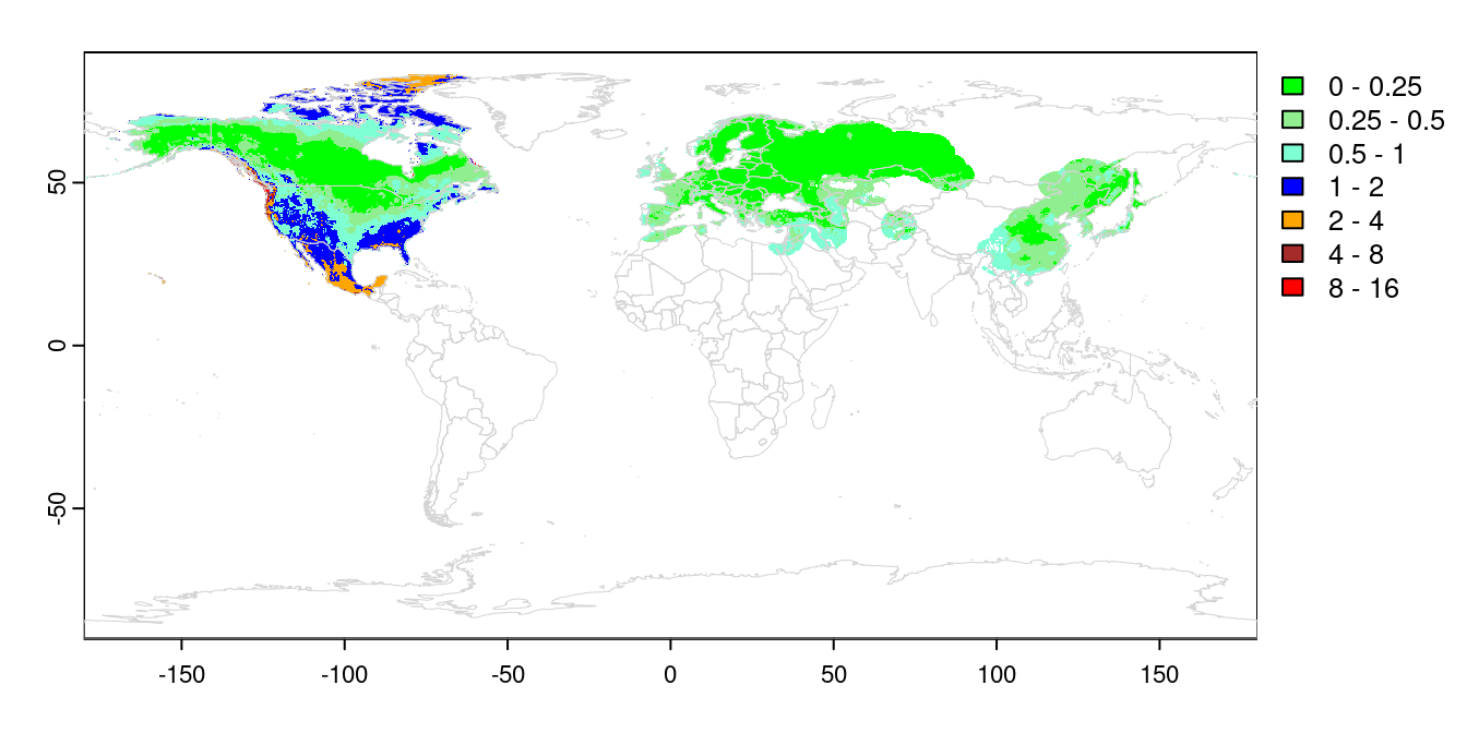
This completes main part of the exDet analysis. We can see the training
range all falls within the range 0-1, which is by design. Transferring that
distribution to North America, we can see most of Canada and the north
central US falls within the same range. The high arctic, the SE US and
western US are all outside of the training range, with Mexico even more
novel. Projections into these areas should be treated with caution, or
avoided entirely.
Most Influential Covariate, MIC
While the map above is our primary interest in exDet analysis, we may
want to know which variables are most influential in creating novel
environments. To do this, we need to calculate the distance map repeatedly,
removing one variable at a time. For each cell, we can then identify the
variable that contributes the most to its NT2 index, by calculating the
difference between the distance for all variables, and the distance with
that variable removed.
names(naMahR) <- "all"

## Remove variables one at a time and recalculate distances:

for(V in VARS){
  SEL <- VARS[VARS != V]

  tmpMeans <- colMeans(trainVal[, SEL], na.rm = TRUE)
  tmpVar <- var(trainVal[, SEL], na.rm = TRUE)
  tmpMah <- mahalanobis(trainVal[, SEL], tmpMeans,
                        tmpVar, na.rm = TRUE)

  thresh <- quantile(tmpMah, probs = 0.95, na.rm = TRUE)
  tmpMah[which(tmpMah > thresh)] <- NA
  tmpMax <- max(tmpMah, na.rm = TRUE)

  resMah <- mahalanobis(naVal[, SEL],
                     tmpMeans, tmpVar, na.rm = TRUE)
  resMah <- resMah/tmpMax
  resMahR <- naWC[[1]]

  ## calculate difference from full distance:
  values(resMahR) <- values(naMahR$all) - resMah

  ## add a layer to our NA raster:
  naMahR[[V]] <- resMahR
}

## Find the maximum difference for each cell:
naMaxMah <- max(naMahR[[-1]])
naTest <- naMahR[[-1]] == naMaxMah

## Convert TRUE/FALSE to category numbers:

for(L in seq_along(names(naTest))){
  values(naTest[[L]]) <- values(naTest[[L]]) * L
}

## Collapse layers into a single raster:
naCat <- max(naTest)

## convert to a factor
levs <- data.frame(vals = seq_along(VARS),
                   ## clean up variable names:
                   levels = gsub("wc2.1_10m_", "", VARS))
levels(naCat) <- levs
Now we can visualize which individual variables are contributing most to the NT2 index for each cell:
plot(naCat, xlim = c(-180, -40), ylim = c(10, 90),
     mar = c(2, 2, 4, 5),
     main = "Most Influential Covariate")
plot(wrld, border = 'lightgrey', lwd = 0.5, add = TRUE)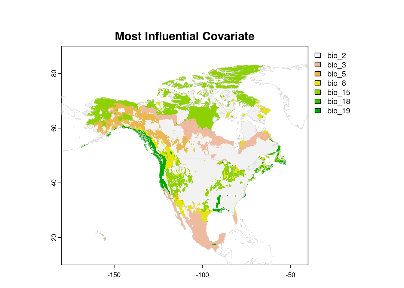
Whether or not that information is useful to you will depend on your research question, of course.
References
Elith, J., M. Kearney, and S. Phillips. 2010. The art of modelling range-shifting species. Methods in Ecology and Evolution 1: 330–342.
Mesgaran, M. B., R. D. Cousens, and B. L. Webber. 2014. Here be dragons: A tool for quantifying novelty due to covariate range and correlation change when projecting species distribution models J. Franklin [ed.], Diversity and Distributions 20: 1147–1159.