Moran’s I

A univariate measure of global spatial autocorrelation.

From Dray, Saïd, and Débias (2008):

\[I(x) = \frac{n\sum_{(2)}c_{ij}(x_i - \bar{x})(x_j - \bar{x})} {\sum_{(2)}c_{ij}\sum_{i=1}^{n}(x_i - \bar{x})^2}\]

where

• \(x_t = [x_1, \dots, x_n]\) is a vector of the variable of interest, which for which spatial coordinates are available
• \(C = [c_{i,j}]\) is a spatial connectivity matrix
• \(\sum_{(2)} = \sum_{i=1}^{n} \sum_{j=1}^{n}\) with \(i \neq j\)

If we define \(z^t = [z_i] = [x_i = \bar{x}]\), the centered variable values, this becomes:

\[I(x) = \frac{n\sum_{(2)}c_{ij}z_iz_j} {\sum_{(2)}c_{ij}\sum_{i=1}^{n}z_i^2}\]

Alternative definition from Wikipedia:

\[I = \frac{N}{W} \frac{\sum_i \sum_j w_{ij}(x_i-\bar{x}) (x_j-\bar{x})} {\sum_i(x_i-\bar{x})^2}\]

• \(N\) is the number of spatial units indexed by \(i\) and \(j\);
• \(x\) is the variable of interest;
• \(\bar x\) is the mean of \(x\);
• \(w_{ij}\) is a matrix of spatial weights with zeroes on the diagonal (i.e., \(w_{ii} = 0\));
• \(W\) is the sum of all \(w_{ij}\).

This is a variation of covariance/correlation, where the contributions of individual comparisons are weighted by the spatial weighting/connectivity matrix.

The value ranges from -1 for complete negative autocorrelation (presence in one cell indicates absence in adjacent cells) to 1 for positive autocorrelation (presence in one cell indicates presence in adjacent cells). 0 indicates no spatial autocorrelation (presence in a cell is unrelated to presences in adjacent cells).

Spatial Weighting Matrix

Can take any form deemed appropriate by the investigator. Binary matrices are often used to limit comparisons to spatially contiguous observations. A common transformation is row-standardization, where elements of the matrix are divided by the sum of their row. Using such a matrix, Moran’s I can be simplified to:

\[ I(x) = \frac{\sum_i\sum_j w_{ij}(x_i - \bar{x})(x_j - \bar{x})} {\sum_i(x_i - \bar{x})^2} \]

Thioulouse et al. (2018) describe options in detail, and include walk-throughs of the main steps in R, based on the spdep package:

1. Create a spatial neighbourhood object (class nb), using criteria of distance (dnearneigh), adjacent polygons (poly2nb), ‘rook’ or ‘queen’ patterns on a grid (cell2nb), or nearest neighbours (knearneigh, which can be asymmetrical). More complex approaches include Delaunay Triangulation (deldir::tri2nb) and Gabriel Graphs (gabrielneigh), which are described in detail by (Legendre and Legendre 2012).

2. Spatial Neighbourhoods (nb) are converted to Spatial Weighting Matrices (class listw). These allows for binary associations to be weighted by spatial distances, including tranformations such as row or total standardization.

Applying spatial weights to the neighbourhood graphs is not clearly explained in the package. This is how it’s done (after Thioulouse et al. 2018)

## Create a neighbourhood network based on
## point-point distance less than MAXDIST 
nbd <- dnearneigh(coords, d1 = 0.001, d2 = MAXDIST)

## calculate inverse distance between observations
invdist <- lapply(nbdists(nbd, coords), function(x) 1/x)

## Apply inverse distances as weights to the
## neighbourhood network:
swm <- nb2listw(nbd, glist = invdist, style = "W")

Adespatial provides the function listw.explore to interactively examine the alternatives available. It didn’t work when I tried it though. Intuitively, creating a neighbourhood based on distance is the most intuitive approach. Neighbourhoods can be edited directly, which might make sense for distributions that span geographic boundaries (ie., lakes or mountains).

Spatial Lag

The spatial lag is a smoothed estimate of the value of a cell, calculated as the weighted averages of all the cell’s neighbours:

\[ \tilde{x}_i = \sum_jw_{ij}x_j \]

Lee (2001) shows Moran’s I is very similar to the Pearson’s correlation between the values of a cell, and the spatial lag for that cell. i.e.,

\[ I(x) = \frac{\sum_i(x_i - \bar{x})(\tilde{x}_i - \bar{x})} {\sqrt{\sum_i(x_i - \bar{x})^2} \sqrt{\sum_i(x_i - \bar{x})^2}} \]

and

\[ r_{X, \tilde{X}} = \frac{\sum_i(x_i - \bar{x}) (\tilde{x}_i - \bar{\tilde{x}})} {\sqrt{\sum_i(x_i - \bar{x})^2} \sqrt{\sum_i(\tilde{x}_i - \bar{\tilde{x}})^2}} \]

It follows that Moran’s I is the correlation between a variable and its spatial lag, scaled by the root of the ratio between the variance of the spatial lag and the variance of the original variable. (really it does, see Lee (2001) for the math). This ratio is the “spatial smoothing scalar,” aka SSS, or at least it is when the spatial weighting matrix is row-standardized.

SSS thus measures the degree of smoothing of a variable when it is represented by its spatial lag. Spatial clustering produces larger SSS values, because increased clustering reduces the difference between a variable and its spatial lag (i.e., increases correlation). The SSS value can be interpreted as the reduction in variance in the spatial lag relative to the original variable.

Together, this allows us to decompose Moran’s I into a correlation value, and a measure of variance reduction (SSS).

Geary’s c

All the papers and books about this stuff mention Geary’s c. It doesn’t appear to be used in any of the analyses, but since everyone else is talking about it, I will too.

\[c(x) = \frac{(n - 1)\sum_{(2)}c_{ij}(x_i - x_j)^2} {2\sum_{(2)}c_{ij}\sum_{i=1}^n(x_i - \bar{x})^2}\]

From Wikipedia, Geary’s c is sensitive to local spatial autocorrelation, capturing relationships among adjacent observations. This contrasts with Moran’s I, which is a measure of global spatial autocorrelation. The two measures are related, but not exactly inverse of each other.

Geary’s c ranges from 0 (positive spatial autocorrelation) to 1 (no spatial autocorrelation) to values larger than 1 (negative autocorrelation).

Co-inertia Analysis

Co-inertia analysis is a form of symmetrical canonical ordination. It is closely related to Procrustes Analysis, and has some parallels to Canonical Correlation Analysis (Legendre and Legendre 2012).

Legendre and Legendre (2012): “variables of both data sets are projected onto the axes obtained by eigen-analysis of the cross-set covariance matrix.” The total co-inertia is the sum of the squared cross-set covariances. The original objects are projected into the co-inertial space. Since each sample is represented in both data sets, we can then compare their relative location in the co-inertial space. Paired observations that are close to each other in this projection indicate that they have similar relative positions in both data sets (“good agreement between” data sets, Thioulouse et al. 2018). Similarly, points that are close together in one data set, but have diverging arrows, indicate similarities in the first data set are not reflected in similarities in the second.

Full details in (Dray, Chessel, and Thioulouse 2003; Dray, Saïd, and Débias 2008; Thioulouse et al. 2018). Very heavy on matrix algebra, hard to develop an intuitive understanding. For the moment, I shall hum along and pretend it is just CCorA.

Spatial Principal Components Analysis

sPCA is the application of co-inertia analysis to a data matrix and its spatial lag. This is a specific case of MULTISPATI, developed particularly for application in population genetics. adegenet::spca() is a high-level wrapper that handles the details, but also obscures some of the steps.

In the case of a genpop object, it does the following:

## Extract the allel frequences from the genpop object:
X <- tab(obj, freq = TRUE, NA.method = "mean")

## coordinates retrieved from the genpop or nb object, or
## supplied by the user:
xy

## regular pca of allele frequencies, default center = TRUE,
## scale = FALSE:
x_pca <- ade4::dudi.pca(x, center = center, scale = scale,
                       scannf = FALSE) 

## Connection network from user or generated interactively:
resCN

## defaults
## scannf = TRUE, nfposi = 1, nfnega = 1

out <- ade4::multispati(dudi = x_pca, listw = resCN,
                       scannf = scannf, nfposi = nfposi,
                       nfnega = nfnega)

This returns an object of class spca, which contains:

eig:

a numeric vector of eigenvalues.

nfposi:

an integer giving the number of global structures retained.

nfnega:

an integer giving the number of local structures retained.

c1:

a data.frame of alleles loadings for each axis.

li:

a data.frame of row (individuals or populations) coordinates onto the sPCA axes.

ls:

a data.frame of lag vectors of the row coordinates; useful to clarify maps of global scores.

as:

a data.frame giving the coordinates of the PCA axes onto the sPCA axes.

call:

the matched call.

xy:

a matrix of spatial coordinates.

lw:

a list of spatial weights of class listw.

tab:

the original data supplied to the PCA (possibly scaled/centered)

Note that the PCA here is based on allele frequencies, which define a Euclidean distance among populations (T. Jombart et al. 2008).

Example:

library(adegenet)
library(utils)
library(graphics)
data(spcaIllus)
spca2A <- spca(spcaIllus$dat2A,
              xy = spcaIllus$dat2A$other$xy, ask=FALSE,
              type = 1, plot = FALSE, scannf = FALSE,
              nfposi = 2, nfnega = 0) 

spca always warns that it is deprecated. The package author says that’s ok, and it should be, since behind the scenes it just calls the function the warning tells you to use anyways.

li contains the observations, projected onto the coinertia space. ls provides the lagged values in the same space. We can compare them using arrows:

plot(spca2A$li, pch = 16, asp = 1)
arrows(x0 = spca2A$li[, 1], x1 = spca2A$ls[, 1],
       y0 = spca2A$li[, 2], y1 = spca2A$ls[, 2],
       length = 0.1)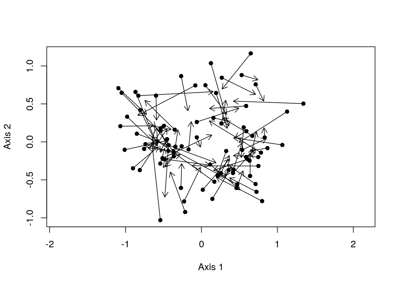

Here, pairs with short arrows indicate sites where the composition of the site is well-described by the composition of its neighbours; they demonstrate high spatial-autocorrelation. In contrast, long arrows denote sites where the actual composition of the site differs substantially from what you would expect based on its nearest neighbours.

These plots don’t appear to be used for sPCA, as they are for other co-inertia analyses. Instead, the values from the first axis are plotted geographically, to illustrate the spatial component of the data:

s.value(spca2A$xy, spca2A$li[,1], include.origin = FALSE,
        addaxes = FALSE, clegend = 0, csize = 0.6)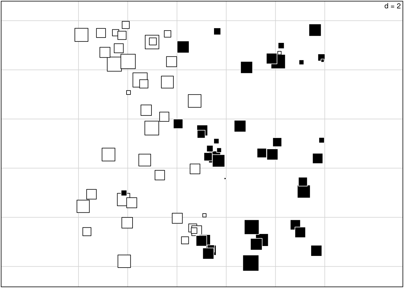 

This shows us the spatial pattern present in the subset of the original data that is spatially structured (on the first axis). We could plot the lagged data the same way, but I’m not sure what that would show us.

We can also contrast this with a spatial plotting of the standard PCA analysis:

allFreq <- tab(spcaIllus$dat2A, freq = TRUE)

pca <- ade4::dudi.pca(allFreq, center = TRUE, scale = FALSE,
                     scannf = FALSE) 

s.value(spca2A$xy, pca$li[,1], include.origin = FALSE,
        addaxes = FALSE, clegend = 0, csize = 0.6)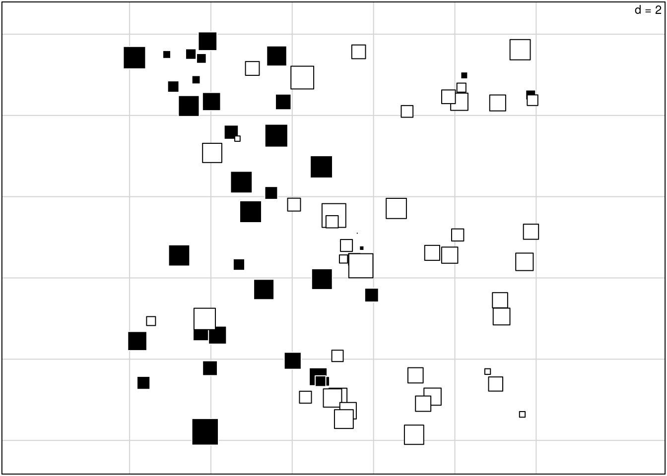 

The main difference is that the sPCA more clearly shows the spatial pattern; that’s what it does. It isolates the spatial pattern in the data, and discards non-spatial structure. There should be a way to quantify how much of the original variation is spatially structured?

Eigenvalues

From Thibaut Jombart (2008): Regular PCA decomposes total variance into decreasing, orthogonal components. sPCA (and MULTISPATI generally, I think) does something different. The eigenvalues are the product of variance and autocorrelation. Axes with high variance and positive autocorrelation indicate strong global structures. That is, they capture a relatively high proportion of the variation in the data, and it has a relatively high proportion of spatial structure (gradient, clustering etc). Axes with low variance represent only a small amount of the total variation, and so aren’t very interesting.

Axes with high variance but high negative autocorrelation indicate strong local structures in the data. That is, spatial replusion, where neighbouring locations are more likely to have different compositions (alleles, species composition etc).

Deciding which axes are interesting seems to be a bit of an art. In general, we look for a large drop between the first or second (or more) axes and the rest, to indicate which ones are worth examining. And similarly at the negative end. The adegenet package (Thibaut Jombart 2008) provides the function screeplot for jointly visualizing the variance and spatial component. Axes that are separated from the main cloud of points are considered interesting/interpretable:

library(stats)
screeplot(spca2A)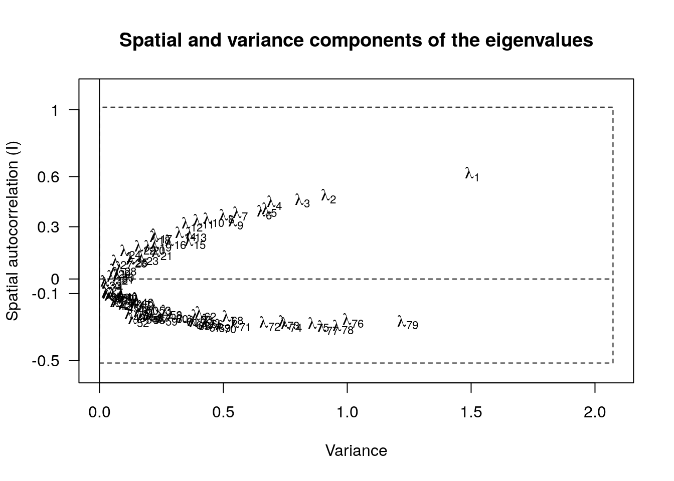

Here, axis 1 is clearly separated, and should be interpreted. Axis 79 is less obvious. And the idea of spatial repulsion is going to be difficult to interpret biologically in most cases I think.

Packaging Oddities & Significance Testing

Note that despite both packages bearing the prefix ade, adespatial and ade4 do NOT use the same implemenatation of co-inertia analysis. ade4 provides the function coinertia() to compute co-inertia on any two data sets. adespatial implements it’s own co-inertia code within the function multispati. The package adegenet provides the wrapper spca, which uses multispati to complete the coinertia analysis it needs. Using the function spca generates a warning, indicating that this function is deprecated and the user ought to use multispati instead. However, spca actually calls multispati itself, so its really just a convenience/wrapper.

The consequence of this is analyses completed via spca and multispati do not return (or contain) an object of class coinertia, and functions in ade4 that process such objects won’t work on their output. Particularly the function ade4::randtest, which might otherwise provide a signficance test for the existence of spatial structure in the data.

But wait! There is a function global.rtest that does provide a randomization test for sPCA objects, and packages the results in a randtest object. It is based on Moran’s Eigenvector Maps. MEMs are part of an alternative approach to spatial ordination from the Legendre group. So, I’m not sure if this is actually testing the significance of the sPCA (i.e., coinertia between the data and its spatial lag matrix), or rather the equivalent in the MEM framework?

Both adespatial and adegenet have their own version of global.rtest, of course. They are nearly identical, but use different code to generate the MEM values. The results are close, but not identical. Can’t say if this is an artifact of them being randomization tests, or if there’s some substantive difference in the implementation.

The co-existence of multiple loosely-loosely linked packages with overlapping/duplicated functions and documentation scattered in books, online tutorials, and, only secondarily, in the package documentation itself, makes figuring this out more work than it needs to be.