Reference
See the RSpatial tutorial for a more detailed introduction/overview of using R for GIS/spatial analysis. The following tutorial walks through some common plotting tasks I use for distribution models.
Basemaps
The raster package provides the function getData, which is a handy way to download basemaps for plotting. (You can also use it to get WorldClim data, see the man page). The first time you call it, it will download the requested maps from the internet. It will save the data in your working directory, or in a location specified with the path argument. The next time you request the same map from getData, if it finds it in the local directory it will load it from there, rather than downloading it again.
library(raster)
us <- getData("GADM", country = "USA", level = 1,
             path = "./data/maps/")
canada <- getData("GADM", country = "CAN", level = 1,
                 path = "./data/maps")
These maps can be plotted directly with the plot command. If you want to combine them, use the add = TRUE argument to the second plot call:
plot(us)
plot(canada, add = TRUE)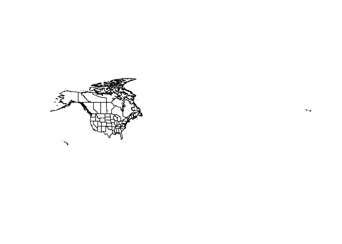
You can combine multiple vector maps into a single map with bind:
na <- bind(us, canada)These maps are 'unprojected', meaning they are plotted in latitude/longitude degrees. That makes it easy to set the plot boundaries:
plot(na, xlim = c(-100, -50), ylim = c(30, 60))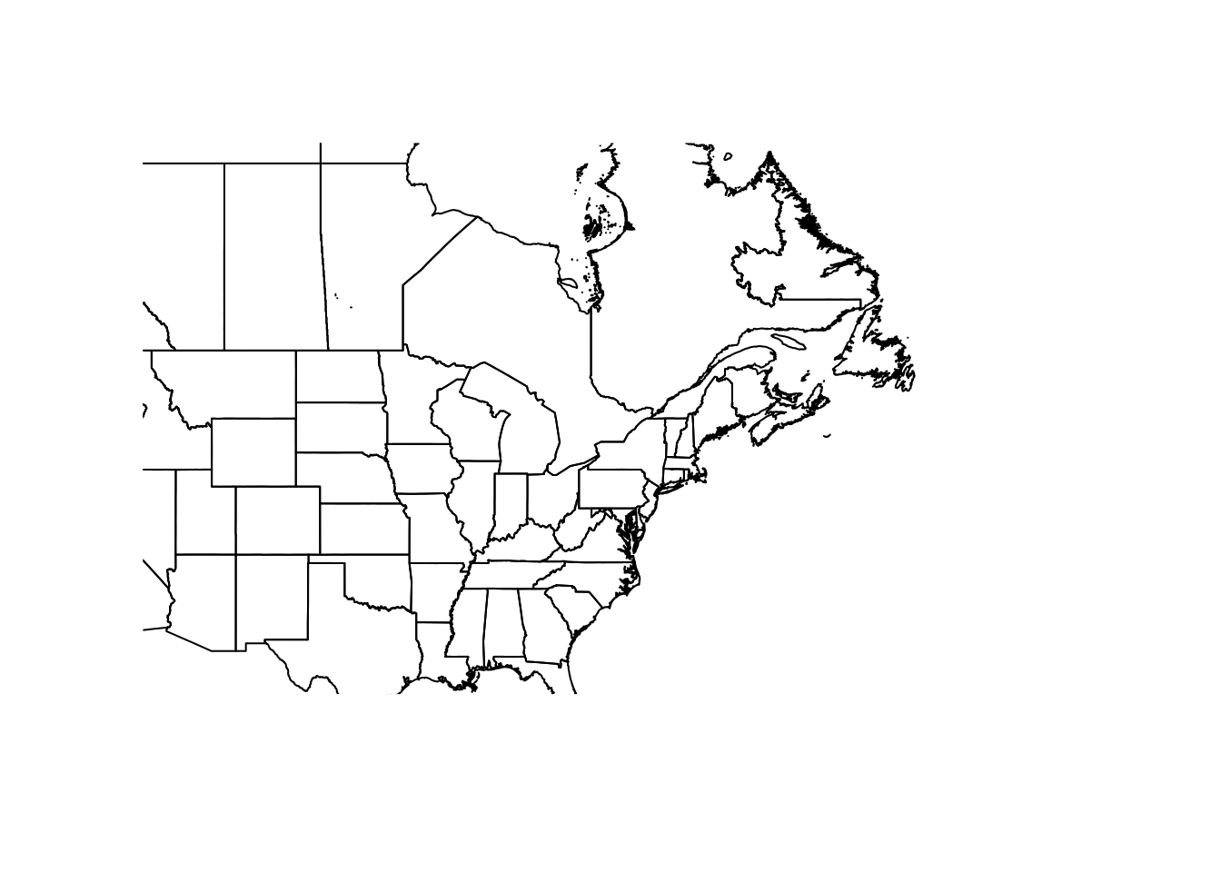
NB: The size of your plot canvas is fixed, but a map can't stretch. The x and y dimensions have to maintain the same aspect. That means zooming in one dimension (i.e. latitude only) won't necessarily change the zoom of your map, if the other dimension fills the canvas. You'll have to play around with the plot size, and both x and y dimensions together, to tweak your zoom.
It's handy to have a shapefile of the Great Lakes, for making prettier maps. I created this one in QGIS and use it for plotting:
greatlakes <- shapefile("data/maps/greatlakes.shp")Adding Data
You can add points to the plot like a regular scatter plot:
library(scales)  ## for the alpha function below
gbif <- read.table("data/trich-gbif.csv")
## Set the line color to gray to focus on the data points:
plot(na, xlim = c(-100, -50), ylim = c(30, 60),
     border = "gray")
points(gbif$X, gbif$Y, pch = 16,
       col = alpha("green", 0.2))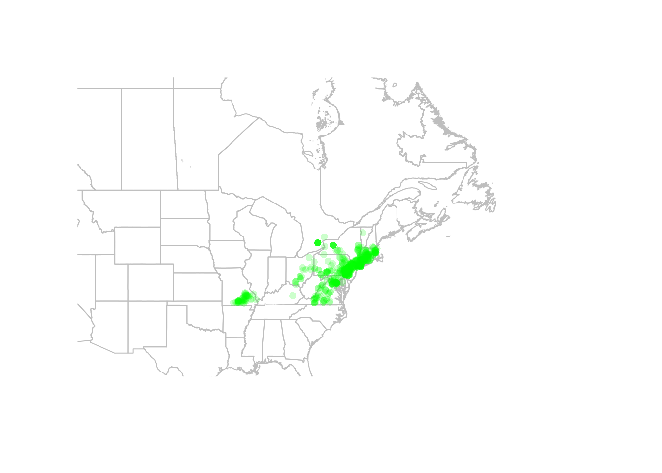
You can also convert your points to a spatial points object, in which case R will know which columns to use for plotting. This is also necessary before we can project our data (see below).
coordinates(gbif) <- ~X+Y
## plot(na, xlim = c(-100, -50), ylim = c(30, 60),
##      border = "gray")
## points(gbif, pch = 16, col = alpha("green", 0.2))
Rasters
Similarly, you can plot rasters with plot:
trichPreds <- raster("./data/trichPreds")
plot(trichPreds, xlim = c(-100, -50), ylim = c(30, 60))
plot(na, border = "gray", lwd = 0.5, add = TRUE)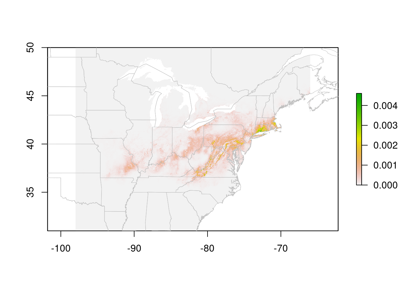
Cells with NA values are transparent. In this case, a species distribution model, low values are displayed in gray. This may be useful for visualizing the extent of the model. However, it looks a bit odd, and makes it hard to see limits of the high-suitability areas. You can tweak this by playing with the color ramp, but it's also handy to 'turn off' the low values entirely (for visualization, not for analysis!!)
trichPredsTrim <- trichPreds
trichPredsTrim[trichPredsTrim <
               quantile(getValues(trichPreds),
                        probs = 0.75, na.rm = TRUE)] <- NA
plot(trichPredsTrim, xlim = c(-100, -50), ylim = c(30, 60))
plot(na, border = "grey", add = TRUE)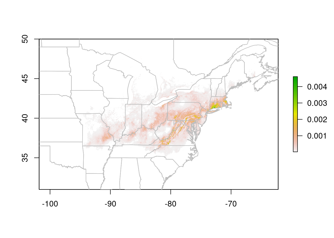
The test I used here, trichPredsTrim < quantile(getValues(trichPreds), probs = 0.75, na.rm = TRUE) identifies all cells in the lower 75% of the suitability scores, which I then set to NA to make them invisible. I decided on 75% after experimenting with different values. In this case, 75% drops most of the grey background (the very lowest values), without eating into the areas that the prediction indicates are suitable.
You could also use an absolute value here, but then you'd need to know the actual distribution of the suitability scores. quantile is easier to tweak.
Projections
Lat/Lon maps look a bit square; we're more used to seeing maps projected. A common projection for Canada is Lambert Conformal Conic. We can transform our data to this projection to make nicer maps:
## define the projection
canlam <- CRS("+proj=lcc +lat_1=49 +lat_2=77 +lat_0=49 +lon_0=-95 +x_0=0 +y_0=0 +datum=NAD83 +units=m +no_defs")

## project our vector data:
na.lcc <- spTransform(na, canlam)
gl.lcc <- spTransform(greatlakes, canlam)

## We already convereted gbif to spatial points object above!
## Now we to set the projection of our points:
crs(gbif) <- CRS("+proj=longlat +datum=WGS84")

## Finally, we can project our points to LCC:
gbif.lcc <- spTransform(gbif, canlam)
Note that our data needs to be in an object of class Spatial*, and it must have a defined coordinate reference system (CRS) before we can project it to a new CRS. Setting the coordinates of our points via the coordinates function creates a Spatial* object. The crs function allows us to explicitly set the projection. We need to know the EPSG code for the projection to use this. The function make_EPSG in the package rgdal is helpful for finding this information. See the RSpatial tutorial for details.
There are a few more steps for raster layers:
rasterLCC <- projectExtent(trichPredsTrim, canlam)
res(rasterLCC) <- 10000 ## set the cell size to 10km
predLCC <- projectRaster(trichPredsTrim, rasterLCC)
Note that I set the resolution to 10km here. That's the size of the raster cells. The original raster cells, in the lat/lon projection, were at 30 second resolution, which is about 1km. I could have set a smaller cell size here. However, since I'm only using this map for visualization, 10km is plenty big enough for my plot, and will run faster (and take less memory) than a map with 1km cell size.
Now we can plot our data in the Lambert Conformal Projection:
plot(predLCC)
plot(na.lcc, border = "grey", add = TRUE)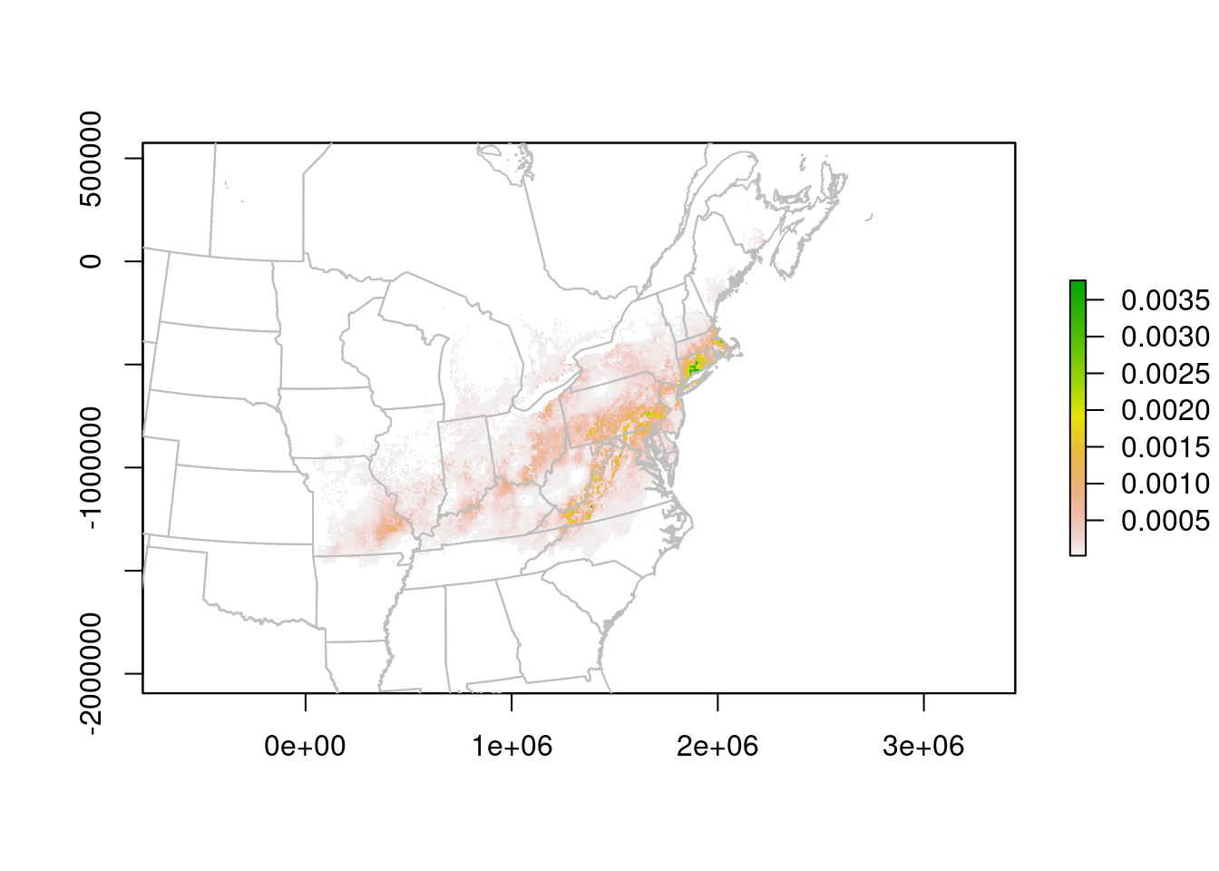
The units are no longer Lat/Lon, but meters. We can read them off the plot to improve the zoom:
plot(predLCC, xlim = c(0, 2500000),
     ylim = c(-1500000, -400000))
plot(na.lcc, border = "grey", add = TRUE)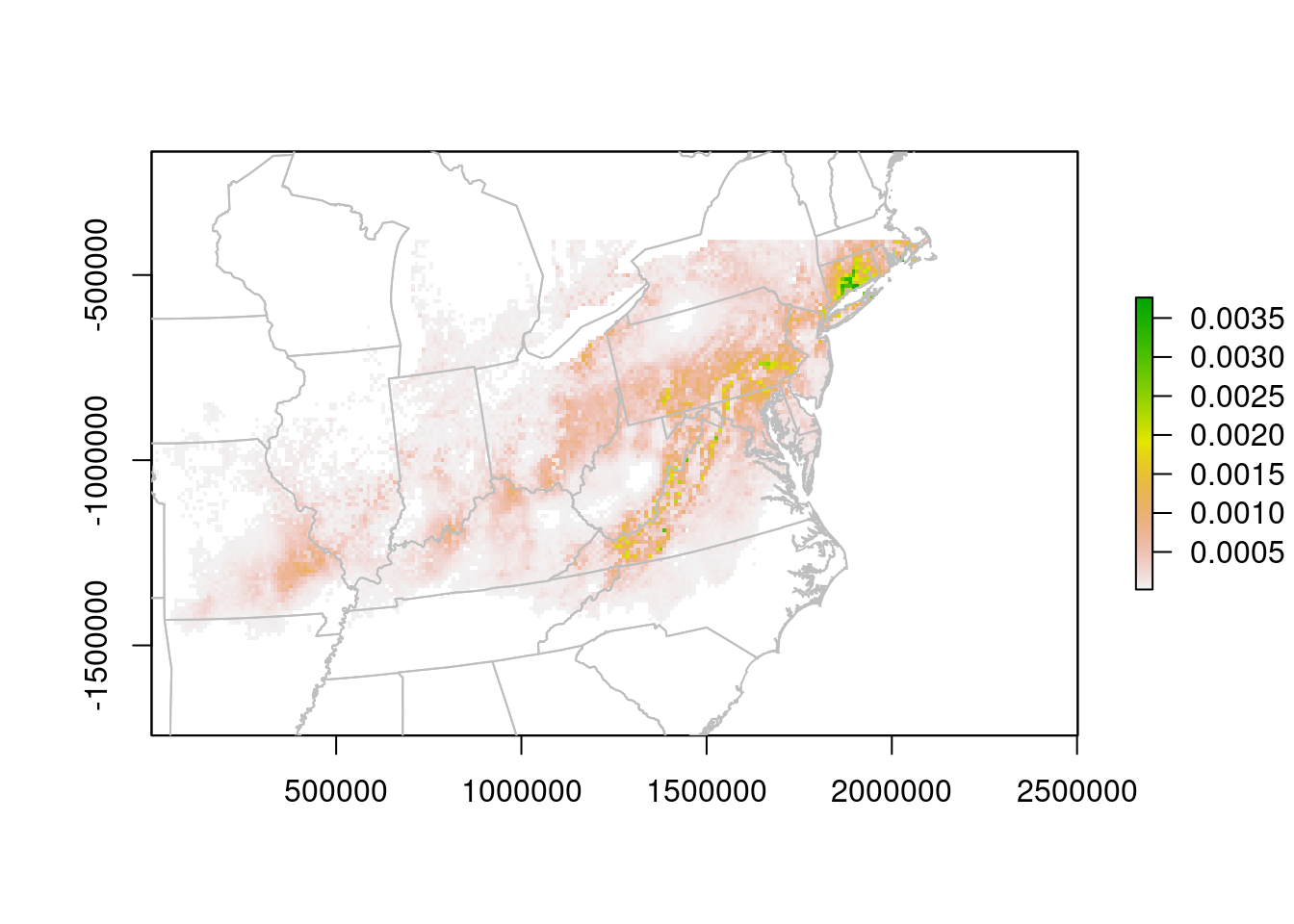
Formatting
With the data plotted, we can then turn to making the map a little prettier:
## Make a panel with two plots, set the right margin tight:
par(mar = c(0.1,0.1,0.1,0), mfrow = c(1, 2))

## store the plot limits:
my_xlims <- c(0, 2500000)
my_ylims <- c(-1300000, -200000)

## Plot the points:
plot(na.lcc, xlim = my_xlims , ylim = my_ylims,
     border = "grey", bg = "lightblue", col = "white")
plot(gl.lcc, add = TRUE, border = "grey", col = "lightblue")
points(gbif.lcc, pch = 16, col = alpha("grey30", 0.2),
       cex = 0.7)
box()

## tighten up the left margin:
par(mar = c(0.1,0,0.1,0.1))
plot(na.lcc, xlim = my_xlims , ylim = my_ylims,
     border = "grey", bg = "lightblue", col = "white")
plot(gl.lcc, add = TRUE, border = "grey", col = "lightblue")
plot(predLCC, add = TRUE, legend = FALSE)

## plotted again to put the border lines on top:
plot(na.lcc, border = "grey", add = TRUE)
box()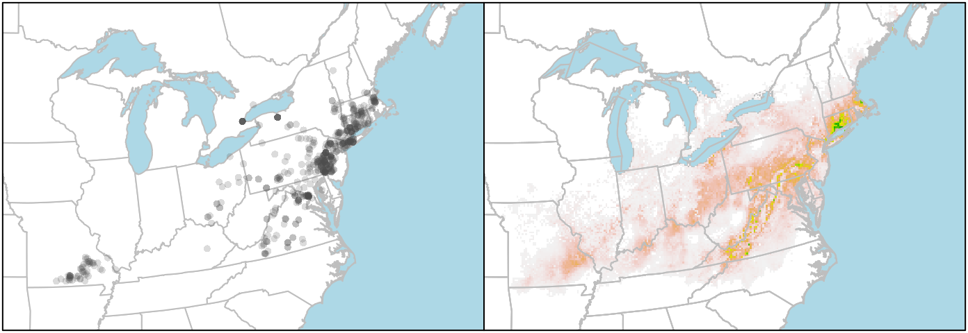
If you want to plot the state/provincial borders on top of the raster, you need to add those layers last. But you can't set the background colour of the raster layer to "lightblue" (or at least I haven't figured that out), so the ocean stays white. I get around that by plotting the boundaries twice, first to set the background colour, and then to put the state lines on top of the raster.