Note that this tutorial refers to the thinning method used in the old version of the rspatial.org tutorial, which used the raster package (along with dismo) for the GIS computations. The terra package will shortly be replacing raster, and all new code should use this instead. The details of spatial thinning with terra are presented in my new ecospat tutorial

A common approach to reducing spatial bias in occurrence records is to randomly select one (or a small number) of samples present in each cell in the landscape. This uses the gridSample function from the package dismo (Hijmans et al. 2017), as described at RSpatial.org.

However, the code presented at RSpatial uses a newly-created raster layer to thin the records. This layer is based on the extent of your occurrence data; even if you set the resolution to match the resolution of the environmental rasters you use, the they won’t necessarily be aligned. That means the cells will be the same size, but the edges won’t line up.

A consequence of this is that you might end up keeping more than one sample, or removing all samples, from a single cell in your environmental data, even after thinning to one sample per cell in your newly-created raster. This lead to some strange behaviour in one of my downstream analyses, where the results for a small data set changed each time I reran the analysis.

I’ll demonstrate using the example from RSpatial:

library(dismo)
library(maptools)
library(sp)
library(raster)

wclim <- getData("worldclim", var = "bio", res = 10,
                path = "../data")

## Warning in getData("worldclim", var = "bio", res = 10, path = "../data"): getData will be removed in a future version of raster
## . Please use the geodata package instead

wc1 <- wclim[[1]]

## crop the climate data to speed up grid creation
wc1crop <- crop(wc1, extent(c(-70, -60),
                           ylim = c(-20, -10)))

data(acaule)
data(wrld_simpl)

acgeo <- subset(acaule, !is.na(lon) & !is.na(lat))
dups2 <- duplicated(acgeo[, c('lon', 'lat')])
acg <- acgeo[!dups2, ]
i <- acg$lon > 0 & acg$lat > 0
acg$lon[i] <- -1 * acg$lon[i]
acg$lat[i] <- -1 * acg$lat[i]
acg <- acg[acg$lon < -50 & acg$lat > -50, ]
coordinates(acg) <- ~lon+lat
crs(acg) <- crs(wrld_simpl)

plot(acg, pch = 20)
plot(wclim[[1]], legend = FALSE, add = TRUE)
points(acg, pch = 20)
plot(wrld_simpl, add=T, border='blue', lwd=2)
box()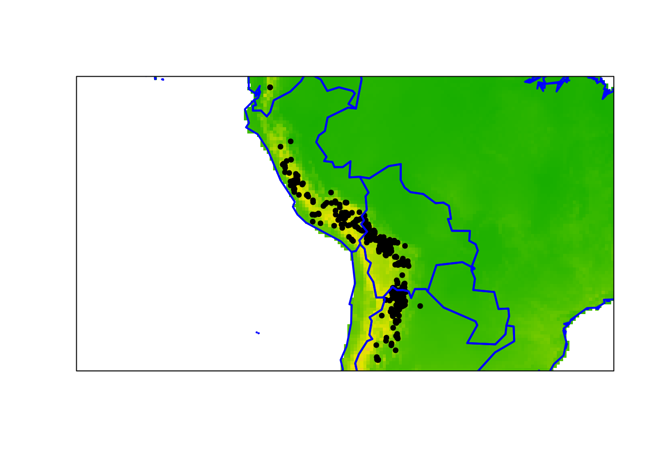

This is the same example from RSpatial. See the link above for more details.

Now we want to thin our records, such that we retain only one observation for each cell in the WorldClim climate layer. To track what’s going on here, I’ll zoom in on one of the crowed areas:

plot(acg, pch = 20, xlim = c(-68.5, -67),
     ylim = c(-17.5, -16.5))
plot(wc1crop, legend = FALSE, add = TRUE)
points(acg, pch = 20)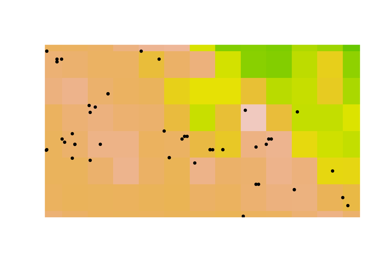

Now lets overlay the grid generated by the code from RSpatial:

r <- raster(acg)
# set the resolution of the cells to the same as wclim
res(r) <- res(wclim)
# expand (extend) the extent of the RasterLayer a little
r <- extend(r, extent(r)+1)
p <- rasterToPolygons(r)

plot(acg, pch = 20, xlim = c(-68.5, -67),
     ylim = c(-17.5, -16.5))
plot(wc1crop, legend = FALSE, add = TRUE)
points(acg, pch = 20)
plot(p, add = TRUE)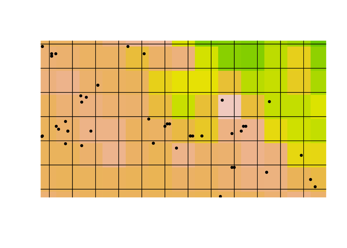

Notice how the climate cells (the coloured squares) are offset from the sampling grid (the black gridlines).

Using this grid for gridSample. I’ll plot a blue ring around the retained occurrences; the records we drop are left as points:

set.seed(1)
acsel <- gridSample(acg, r, n=1)

plot(acg, pch = 20, xlim = c(-68.5, -67),
     ylim = c(-17.5, -16.5))
plot(wc1crop, legend = FALSE, add = TRUE)
points(acg, pch = 20)
plot(p, add = TRUE)
points(acsel, col = 'blue', cex = 2)

Take a close look at that last plot. Notice that there are climate cells with no retained observations:

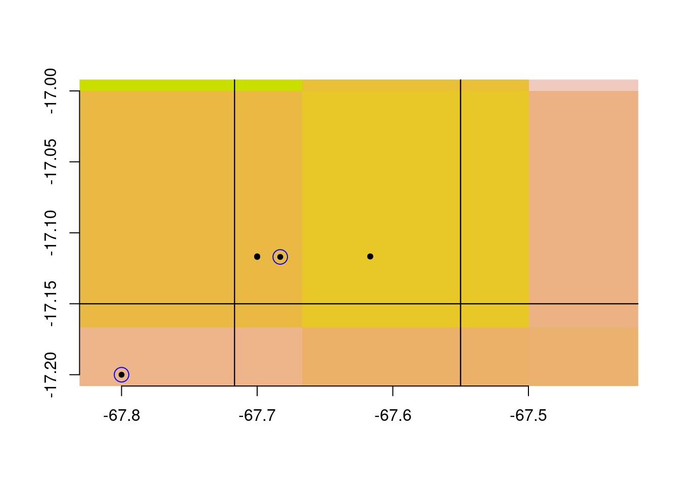
As well as climate cells with multiple observations:

This is fine if you are using the occurrence records in a purely spatial analysis (i.e., without incorporating climate data for each observation). But if you are intending to retain at most one observations for every cell in your climate map, this is not what you were hoping for.

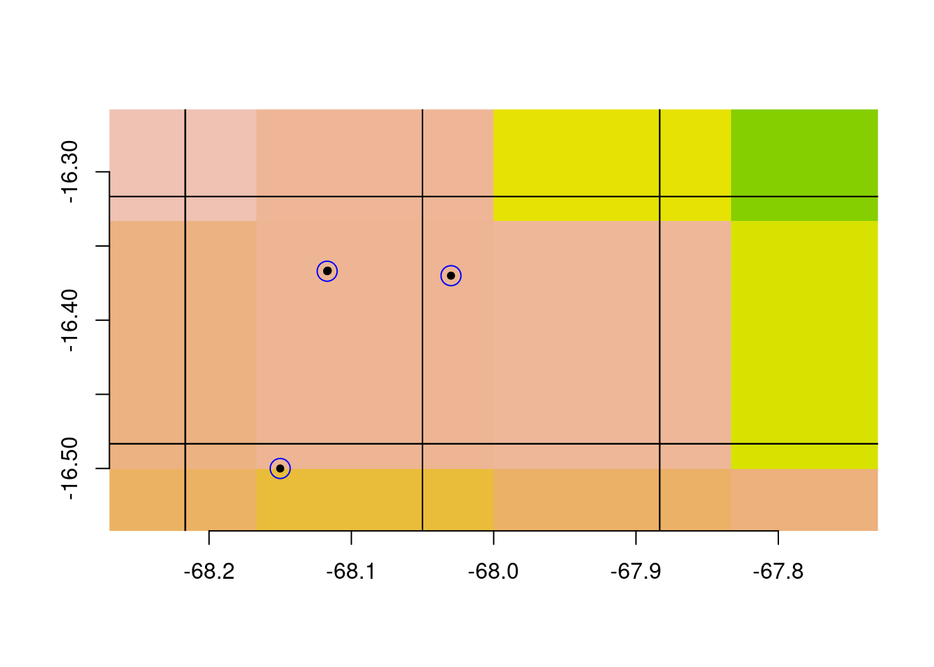
A better way to achieve our desired result is to use the climate layer directly in gridSample:

set.seed(1)
acselClimate <- gridSample(acg, wc1, n=1)

Lets visualize the grid we sampled on:

plot(acg, pch = 20, xlim = c(-68.5, -67),
     ylim = c(-17.5, -16.5))
plot(wc1crop, legend = FALSE, add = TRUE)
points(acg, pch = 20)

## using a cropped layer because this is a slow operation:
climGrid <- rasterToPolygons(wc1crop)
plot(climGrid, add = TRUE)
points(acselClimate, col = 'blue', cex = 2)

Everything matches up as we expect now: the sampling grids are perfectly aligned with the climate cells.

This approach will only work if your climate raster covers the full extent of your occurrence records. Which it really should - if it doesn’t, the records that aren’t covered will end up getting dropped from your analysis since there’s no climate data at those locations.

References

Hijmans, Robert J., Steven Phillips, John Leathwick, and Jane Elith. 2017. “Dismo R Package Version 1.1-4.” https://CRAN.R-project.org/package=dismo.