Key Resources

Merow et al. (2013) provides a very thorough introduction to Maxent modeling, and especially to what the various settings mean and how to set them.

RSpatial is a (nearly complete) set of lessons covering spatial data analysis in R, and including good tutorials for Maxent and other SDM approaches.

Best Practices in Species Distribution Modeling in R is another set of online notes. I have reviewed them briefly, and they look to be very thorough.

From the same author (Adam B. Smith), a webinar on using herbarium data in ecology, evolution and conservation, and a database of biodiversity databases.

Another workshop, from Lee-Yaw, is available on github. It’s a little old now, and doesn’t appear to be as comprehensive as Smith’s workshop above (maybe?). However, some people may prefer the more condensed format. Both authors have demonstrated expertise in the subject, so I don’t doubt that these are both reliable sources.

Sampling Bias

Sampling bias in occurrence data is an issue because it means we can’t be sure a species is detected under certain conditions because that’s it’s preferred habitat, or because those are the conditions in the locations we prefer to search.

“The uniform sampling assumption does not require a uniformly random sample from geographic space, but instead that environmental conditions are sampled in proportion to their availability, regardless of their spatial pattern” (Merow et al., 2013).

This problem can be addressed by thinning records (also called spatial filtering, Radosavljevic and Anderson, 2014), such that multiple records from within the same area are represented by only one or a few of the total records. This is a bit crude, but should remove the worst biases, such as a particular field station getting preferentially sampled by recurring visits from scientists or students, or general biases towards sampling roadsides and popular trails.

Lee‐Yaw et al. (2018) developed their own method to thin species records, using kernel smoothing estimates to reduce the number of samples from a neighbourhood, and selecting which samples to keep via novel environments. I don’t think this is widespread, and feels a bit like overkill.

Another interesting approach in Atwater et al. (2018), who used a large dataset of gbif records to establish geographic (and presumably also environmental) bias in the full set of records, and used that to correct bias for individual species. Simply put, occurrence records for each species are weighted by the proportion of records for the entire set are found in that location (either geographic or a cell in a climate grid).

Subsampling based on raster grids is a simpler, more intuitive approach provided by Hijmans et al. (2017). It doesn’t account for the possibility that local density may be an accurate reflection of the niche requirements of a species, as the approach of Lee‐Yaw et al. (2018) does.

NB: See my extended discussion of thinning records on a grid

Grid-sampling:

### create an empty raster
r <- raster::raster(trich) 
###  set the resolution:
###   to match the environmental layers
res(r) <- res(env)

###   to set to one minute, ca 2km square
res(r) <- 1/60 

###   double the environmental layer
res(r) <- 2 * res(env) 

### IMPORTANT: extend it outwards one cell
### otherwise, points at the edge of the range
### might get dropped!!

### NB: use the `snap = "out"` argument to ensure the extent
### limits 'round up' (or round out) to the next full cell
### row/column. Without this, in some circumstances extent +
### 1 'snaps back' to the original extent.
r <- extend(r, extent(r) + 1, snap = "out") 

### sample one point per cell:
trichsel <- gridSample(trich, r, n = 1) 

Aiello‐Lammens et al. (2015) provides an alternative approach based on imposing a minimum permissible nearest-neighbour distance, and then finding the set that retains the most samples through repeated random samples.

Thinning by Nearest-Neighbour:

## thin.par sets minimum distance in km
trichthin <- thin(data.frame(LAT = coordinates(trich)[, "Y"],
                             LONG = coordinates(trich)[, "X"],
                             SPEC = rep("tplan", nrow(trich))),
                  thin.par = 2, reps = 1, write.files = FALSE,
                  locs.thinned.list.return = TRUE) 

Radosavljevic and Anderson (2014) show that unfiltered/unthinned data produces elevated assessment of model performance, as a consequence of over-fitting to spatially auto-correlated data. So filtering works.

See also Boria et al. 2014, Varela et al. 2014 (unread)

Merow et al. (2013) provide two more rigorous approaches, depending on whether or not data on search effort is available. When search effort is known, it can be used to construct a biased prior.

When search effort is unknown, we can create a biased background sample to account for bias in presence data, via Target Group Sampling. Under TGS, records that are collected using the same surveys/methods as the focal species are form the background points. i.e., the set of all herbarium records in GBIF may be an appropriately biased background for any one of those plant species. This assumes that the target plant is collected/detected at the same rate as the reference set. It may be appropriate to subset the reference set to increase the likelihood of this being true: use only graminoids as biased background for sedges, or woody plants as background for a tree?

Spatial Bias

Elith, Phillips, et al. (2010) – The area of individual cells in raster layers projected in Lat-Lon coordinates are not equal. This can be corrected by:

• project the grids to an equal area projection
• create a ‘bias grid’ that can be used to weight background samples
• create a background sample with appropriate sampling weights

Study Extent

Discussed extensively in Barve et al. (2011). They identified three general approaches to consider:

1. Biotic regions (ecozones etc). A good compromise between biological realism and tractability
2. Niche-model reconstructions: back-project a niche model over the appropriate time period (i.e., previous glacial maximum or interglacial) to identify the area that the species could have occupied over an extended period. Nice idea, but a real risk of circularity?
3. Detailed simulations. Sounds great, but I think if we had enough data to properly parameterize such a model, we wouldn’t need to resort to sdms in the first place.

If you wanted to improve on biotic regions, things to consider in developing a more rigorous approach should include:

1. Dispersal characteristics of the species
2. Crude estimate of the niche (again, circularity?)
3. Establish relevant time span
4. Identify relevant environmental changes

Soberón (2010) is often cited together with Barve et al. (2011), but the latter provides more explicit discussion of best practices for sdm model construction. I think the deference to Soberon is probably due to their creation of the BAM model (in earlier publications), which Barve’s system is based on (Biotic, Abiotic, Movement).

Merow et al. (2013) provide a shorter discussion, and emphasize matching the study extent to the biological question of interest. Prioritizing sites for protection within the range of a species should constrain the extent to the existing range of the species; evaluating invasion potential should use an extent large enough to encompass the areas of concern (i.e., global, or continental scale for novel invasives).

Variable Selection

Variables == predictors, the spatial layers used as the environmental/dependent variables in the model.

Interesting discussion in Guisan et al. (2017) (section 6.4, page 102+): variables that are measured most accurately often/usually are only indirectly related to a species’ niche; e.g., elevation, slope, aspect. Very precise and accurate spatial layers are available for these.

Variables with a direct relationship to a species niche are usually created through interpolation from sparse reference points (weather stations), and this involves unavoidable error propagation and imprecision.

Over small extents, it may be preferable to use indirect variables, as they offer greater precision in quantifying the local environment. However, as extent increases, the relative value of direct variables increases. The indirect variables are likely not stationary on large scales - a species relationship to slope and elevation are likely different in southern US vs northern Canada, for instance. On the other hand, a species relationship to temperature, however coarsely it is mapped, is likely similar across its geographic range.

Elith, Phillips, et al. (2010) point out that Maxent’s built-in variable selection (via L1-regularization) is reliable, relatively insensitive to correlation among variables, and model performance may actually be degraded by imposing additional model selection procedures prior to running Maxent! They do suggest that sticking to proximal variables is preferable when projecting models to novel contexts.

I will need to reconsider whether evaluating collinearity is something I should continue to do. In the meantime, I leave the following notes on how to do it:

Merow et al. (2013) identify two general approaches to selecting variables. The machine learning approach is based on the understanding that the Maxent algorithm will, by design, select the most useful variables and features, so we can include all reasonable variables.

However, this probably only applies when the objective is to provide accurate predictions of occurrences in the same context in which the model is built. Efforts to understand the environmental constraints on that distribution, or projecting it to a new context, will be potentially confounded when the model includes correlated variables.

To minimize this problem, Merow et al. (2013) recommends taking a statistical approach (i.e., treating a Maxent model as a ‘conventional’ statistical model). In this case, they recommend prescreening variables to limit colinearity, and emphasize biologically relevant variables. This should produce more parsimonious and interpretable models.

Pairwise correlations can be used to identify pairs or groups of variables that are highly correlated. ENMTools (Warren et al., 2019) provides several helper functions for this, including raster.cor.matrix, raster.cor.plot.

I prefer using hclust based on 1 - abs(cor) to visualize correlated groups:

## "predictors" is a raster stack

## Calculate correlations:
cors <- raster.cor.matrix(predictors) # from ENMTools

threshold = 0.7  ## the maximum permissible correlation

dists <- as.dist(1 - abs(cors))

clust <- hclust(dists, method = "single")
groups <- cutree(clust, h = 1 - threshold)

## Visualize groups:
plot(clust, hang = -1)
rect.hclust(clust, h = 1 - threshold)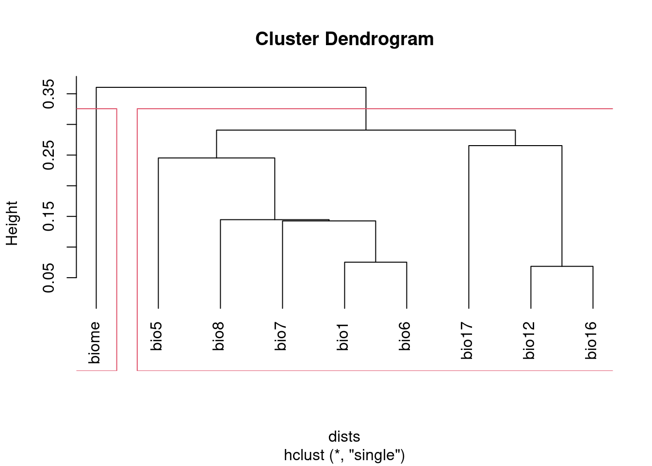

## Print the groups:
groups

##  bio1 bio12 bio16 bio17  bio5  bio6  bio7  bio8 biome 
##     1     1     1     1     1     1     1     1     2

NB I set the method argument to "single". This ensures that all the variables with correlations above the threshold will be captured together in a cluster. The default method, "complete", creates clusters that may include variables with correlations above the specified threshold. See discussion of hierarchical agglomerative clustering (section 8.5) in Legendre and Legendre (2012) for details, if you want to know more.

After running this, groups will identify which cluster each variable belongs to. Keep at most one variable from each group.

This doesn’t absolutely guarantee that variables in different groups will have correlations less than threshold, but in most cases this will be true. When it isn’t, the highest inter-group correlation will still be very close to the threshold. If you’re concerned, double check the correlations of the variables after you’ve picked them.

Alternatively, you can use cutree to select the number of groups you want, then pick a variable from each group. Since this doesn’t use a threshold, you’ll have to make sure the number of groups you pick is equal to or lower than the number of groups generated using the threshold approach.

## "predictors" is a raster stack

## Calculate correlations:
cors <- raster.cor.matrix(predictors) # from ENMTools

groupNum = 3  ## the desired number of groups

dists <- as.dist(1 - abs(cors))

clust <- hclust(dists, method = "single")
groups <- cutree(clust, k = groupNum)

## Visualize groups:
plot(clust, hang = -1)
rect.hclust(clust, k = groupNum)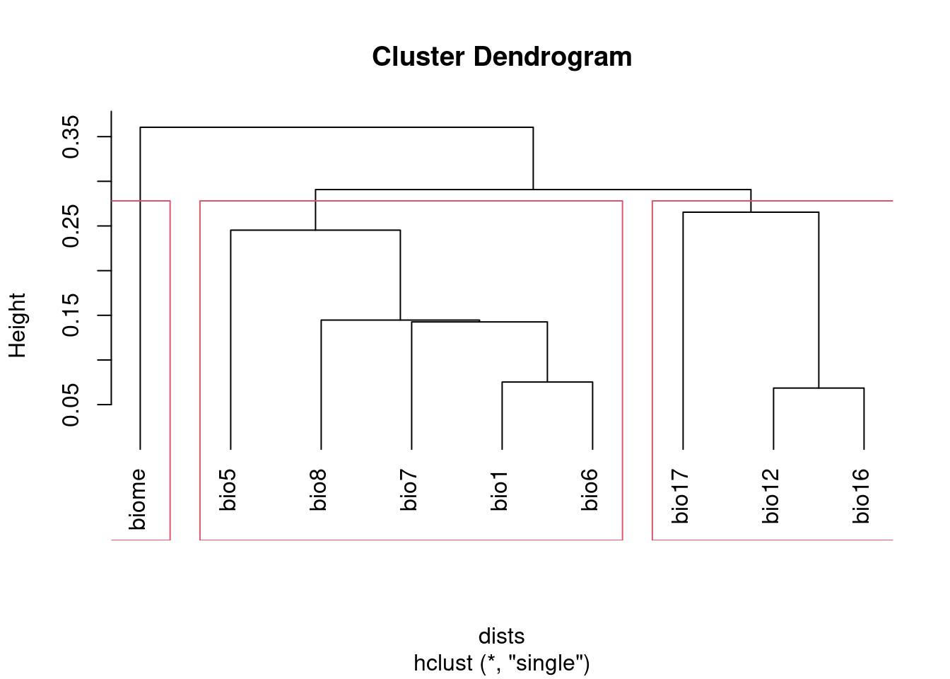

## Print the groups:
groups

##  bio1 bio12 bio16 bio17  bio5  bio6  bio7  bio8 biome 
##     1     2     2     2     1     1     1     1     3

However, neither of these approaches will address multicollinearity among three or more variables. Guisan et al. (2017) suggest using the function usdm::vif instead, which calculates variable inflation. They recommend keeping the vif values under 10, but different authors will use cutoffs from 5-20.

Petitpierre et al. (2017) explicitly tested different approaches to model selection for use in projecting models in space and time. Their results support Merow’s statistical approach: modelers should use a small number of ‘proximal’ variables (i.e., variables known to be biologically relevant to the species in question), or, particularly when very few observations are available for training, the first few PCA axes of a larger set of environmental variables. PCA axes are orthogonal (i.e., not collinear) by construction, but interpretation may be tricky if they incorporate a large number of variables.

Petitpierre et al. (2017) also recommend a suite of “State of the Art” variables, including the familiar bioclim variables annual mean temp, Temp var, Temp coldest quarter, Temp warmest quarter, Precip var, and Precip wet quarter, to which they add two measures of the “moisture index”: annual mean moisture index (Ma), and moisture index seasonality (Mvar). These are available from Climond.org. At a global scale, annual mean temperature and temperature of the warmest quarter are (not suprisingly) highly correlated, and the moisture indices are moderately correlated with precip var and precip wet quarter (again, not suprising). So it might be reasonable to use a reduced set of the State of the Art variables in studies that aim to generate transferable models: Tvar, Tcoldq, Pvar, Pwetq, Mvar.

Note that the Climond data is currently (2023-10-19) only available at 10’ and 30’ resolution, while Worldclim provides data (without the moisture indices) down to 30" resolution.

Feature Selection

Features == the statistical models used to fit the variables to the response variables (presences). i.e., linear, quadratic, product, hinge, threshold, categorical.

Note that hinge is essentially a superset of linear and threshold features, so if you have hinges, the other two are redundant (Elith, Phillips, et al., 2010). As of version 3.4.0, threshold featues are not included by default; experience has shown that this improves model performance, and produces simpler, more realistic models (Phillips et al., 2017). Similarly, product features appear to contribute very little to model performance, given the added complexity.

Merow et al. (2013) recommend selecting features on biological grounds. They provide a short discussion, noting that the fundamental niche is likely quadratic for most variables over a large enough extent, but may be better approximated by a linear function if the study extent is truncated with respect to the species’ tolerance for that variable (ala Whittaker). Interesting ideas, but not much to go on unless you actually do know a fair bit about your species.

Warren and Seifert (2011) describe a process for selecting features to keep/include in the model (linear, quadratic, polynomial, hinge, threshold, categorical). It uses the AIC to identify the optimal combination. Easy and quick to do with the ENMEval package (note that many references cite ENMTools for these tests, but they’ve been moved to ENMEval nowadays).

NB applying different spatial filtering/thinning to your data can produce different ‘optimal’ models (i.e., different retained features and regularization value), as determined by the AIC criterion.

NB The enmeval function only evaluates AIC for models with an appropriate number of parameters. If you have a low number of observations, a low regularization (i.e., permissive approach to including parameters), and complex/high-parameter models (especially hinge features), the AIC values will be reported as NA. These models are overfit, and as such you shouldn’t use them with your data. Explanation on Maxent discussion list.

Regularization

Regularization is used to penalize complexity. Low values will produce models with many predictors and features, with 0 leading to all features and variables being included. This can lead to problems with over-fitting and interpretation. Higher regularization values will lead to ‘smoother’, and hopefully more general and transferable models. There will be a trade-off between over- and under-fitting.

The default values in Maxent are based on empirical tests on a large number of species. These are probably not unreasonable, but it’s pretty standard to mention that they’re a compromise, and we improved them for our the needs of our particular species and context by doing X (for various values of X).

The approach of Warren and Seifert (2011) (see previous) can be used here as well, testing a range of regularization (aka beta) values, and selecting the one that generates the lowest AIC. It may also be worth selecting the simplest model that is within a certain similarity of the ‘best’ model? That’s more to explain to reviewers though.

Warren and Seifert’s simulations demonstrate that models with a similar number of parameters to the true model produce more accurate models, in terms of suitability, variable assessment, and ranking of habitat suitability, both for the training extent and for models projected in space/time. Furthermore, AIC and BIC are the most effective approaches to model tuning to achieve the correct number of parameters.

Radosavljevic and Anderson (2014) also consider the impact of the regularization parameter on over-fitting. They find that the default value often leads to over-fitting, especially when spatial auto-correlation is not accounted for in model fitting. They conclude that regularization should be set deliberately for a study, following the results of experiments exploring a range of potential values.

Note that specifying the regularization is done via the betamultiplier argument, which applies to each of the different feature classes. That is, the actual regularization value will be set by Maxent automatically for each class, subject to the multiplier value specified by the user. We don’t set the regularization values for each class directly (which is possible via the options beta_lqp, beta_threshold etc. (Phillips, 2017), although Radosavljevic and Anderson (2014) suggest experiments to explore this should be done.

Output type

Raw: values are Relative Occurrence Rate (ROR) which will sum to 1 over the extent of the study. Merow et al. (2013) considers this to be a reasonable interperetation of the Maxent output, but the actual values can be difficult to interpret; they produce maps that “do not often match ecologists’ intuition about the distribution of their species” (Phillips et al., 2017).

Logistic: attempts to provide an accurate estimate of the probability that the species is present, given the environment. Monotonically related to raw values; site rank is identical for these measures. Based on the assumption that there is a 50% probability that a species will be present at a site with ‘average’ conditions for the species. This assumption is problematic and unrealistic according to Merow et al. (2013). However, Elith, Phillips, et al. (2010) prefer logistic output, and discuss justification for preferring it over raw values.

Cumulative: the sum of all cells with <= to the raw value of the cell. Rescaled to range from 0-100.

Complementary Log-Log (aka CLOGLOG): the standard output from version 3.4.0 onwards. Generally similar to the logistic output, but tending to give slightly higher values. There is a stronger theoretical justification for CLOGLOG than logistic, as summarized in Phillips et al. (2017). CLOGLOG provides an estimate of the probability of presence, but with the caveat that this probability is based on an arbitrary quadrat size (similar to the prevalence assumption made with logistic).

Merow et al. (2013) recommends sticking to Raw whenever possible, which means using the same species in the same extent. Note that the raw values will change for different extents, even for identical models, so they can’t be compared across projections without additional post-processing.

Cumulative is preferable when defining/describing range boundaries, or otherwise dealing with omission rates.

Elith, Phillips, et al. (2010) prefer to use the logistic, which they present as a biologically reasonable estimate. However, it will be a problem in comparisons among species with different prevalence on the landscape, as it assumes identical (and arbitrary) prevalence.

Following (Phillips et al., 2017), CLOGLOG now seems to be the most intuitive output to use in most cases.

Evaluation

Projection

Complex models, with large numbers of predictors, or that use complex features, are more likely to be overfit. Overfitting sacrifices generality (i.e., capacity to project to different scenarios) in favour of better fit to training data. Consequently, for the purposes of projection, we may want to emphasize smaller, simpler models. See also Petitpierre et al. (2017) for discussion of variable selection.

Guisan et al. (2017): two related issues to consider when comparing the environment in the training region to that in the region into which the model is projected:

• availability: are environment ‘types’ similarly abundant and available?

• analog: are the environment ‘types’ in the projected range also present in the training range?

The act of projection implicitly assumes environments are fully analagous with equal availability.

This is to a large extent unavoidable, so we have to take measures to reduce it in data preparation, and/or account for it in interpretation of results.

Ensembles

TODO

TO-READ

Boria, R. A. et al. 2014. Spatial filtering to reduce sampling bias can improve the performance of ecological niche models. – Ecol. Model. 275: 73–77.

Varela, S. et al. 2014. Environmental filters reduce the effects of sampling bias and improve predictions of ecological niche models. – Ecography 37: 1084–1091.